Wang_ChestX-ray8_Hospital-Scale_Chest_CVPR_2017_paper.pdf

发布时间：2022-05-31 发布人：admin 分类：说明书资料大小：1.57M 资料格式：pdf 举报版权申诉

sinat_24493477-9901744-4744302543297035893.pdf-第1页.png

第1页 / 共10页

sinat_24493477-9901744-4744302543297035893.pdf-第2页.png

第2页 / 共10页

sinat_24493477-9901744-4744302543297035893.pdf-第3页.png

第3页 / 共10页

sinat_24493477-9901744-4744302543297035893.pdf-第4页.png

第4页 / 共10页

sinat_24493477-9901744-4744302543297035893.pdf-第5页.png

第5页 / 共10页

sinat_24493477-9901744-4744302543297035893.pdf-第6页.png

第6页 / 共10页

sinat_24493477-9901744-4744302543297035893.pdf-第7页.png

第7页 / 共10页

sinat_24493477-9901744-4744302543297035893.pdf-第8页.png

第8页 / 共10页

文本预览

ChestX-ray8: Hospital-scale Chest X-ray Database and Benchmarks on Weakly-Supervised Classiﬁcation and Localization of Common Thorax Diseases Xiaosong Wang1, Yifan Peng 2, Le Lu 1, Zhiyong Lu 2, Mohammadhadi Bagheri 1, Ronald M. Summers 1 1Department of Radiology and Imaging Sciences, Clinical Center, 2 National Center for Biotechnology Information, National Library of Medicine, National Institutes of Health, Bethesda, MD 20892 {xiaosong.wang,yifan.peng,le.lu,luzh,mohammad.bagheri,rms}@nih.gov Abstract The chest X-ray is one of the most commonly accessi- ble radiological examinations for screening and diagnosis of many lung diseases. A tremendous number of X-ray imaging studies accompanied by radiological reports are accumulated and stored in many modern hospitals’ Pic- ture Archiving and Communication Systems (PACS). On the other side, it is still an open question how this type of hospital-size knowledge database containing invaluable imaging informatics (i.e., loosely labeled) can be used to fa- cilitate the data-hungry deep learning paradigms in build- ing truly large-scale high precision computer-aided diagno- sis (CAD) systems. In this paper, we present a new chest X-ray database, namely “ChestX-ray8”, which comprises 108,948 frontal- view X-ray images of 32,717 unique patients with the text- mined eight disease image labels (where each image can have multi-labels), from the associated radiological reports using natural language processing. Importantly, we demon- strate that these commonly occurring thoracic diseases can be detected and even spatially-located via a uniﬁed weakly- supervised multi-label image classiﬁcation and disease lo- calization framework, which is validated using our proposed dataset. Although the initial quantitative results are promis- ing as reported, deep convolutional neural network based “reading chest X-rays” (i.e., recognizing and locating the common disease patterns trained with only image-level la- bels) remains a strenuous task for fully-automated high pre- cision CAD systems. 1 Introduction The rapid and tremendous progress has been evidenced in a range of computer vision problems via deep learning and large-scale annotated image datasets [25, 37, 13, 27]. 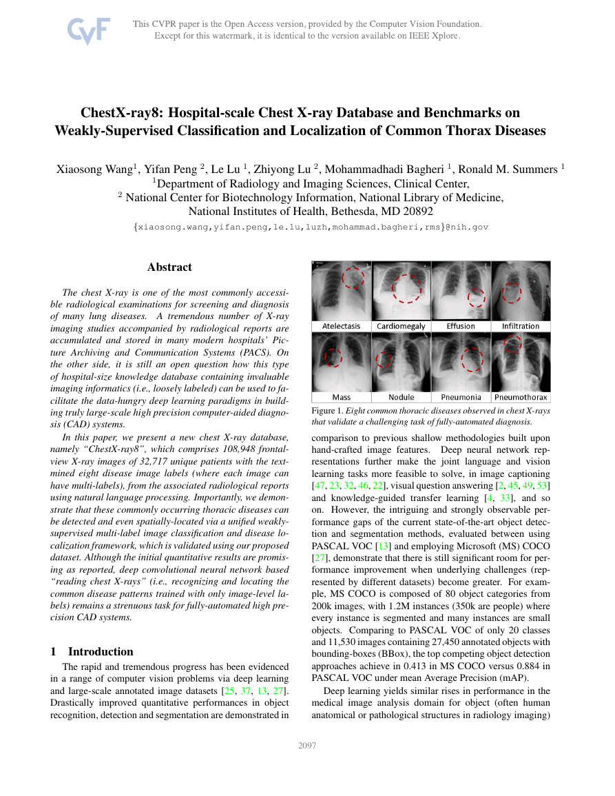Drastically improved quantitative performances in object recognition, detection and segmentation are demonstrated in Figure 1. Eight common thoracic diseases observed in chest X-rays that validate a challenging task of fully-automated diagnosis. comparison to previous shallow methodologies built upon hand-crafted image features. Deep neural network rep- resentations further make the joint language and vision learning tasks more feasible to solve, in image captioning [47, 23, 32, 46, 22], visual question answering [2, 45, 49, 53] and knowledge-guided transfer learning [4, 33], and so on. However, the intriguing and strongly observable per- formance gaps of the current state-of-the-art object detec- tion and segmentation methods, evaluated between using PASCAL VOC [13] and employing Microsoft (MS) COCO [27], demonstrate that there is still signiﬁcant room for per- formance improvement when underlying challenges (rep- resented by different datasets) become greater. For exam- ple, MS COCO is composed of 80 object categories from 200k images, with 1.2M instances (350k are people) where every instance is segmented and many instances are small objects. Comparing to PASCAL VOC of only 20 classes and 11,530 images containing 27,450 annotated objects with bounding-boxes (BBox), the top competing object detection approaches achieve in 0.413 in MS COCO versus 0.884 in PASCAL VOC under mean Average Precision (mAP). Deep learning yields similar rises in performance in the medical image analysis domain for object (often human anatomical or pathological structures in radiology imaging) 12097

detection and segmentation tasks. Recent notable work in- cludes (but do not limit to) an overview review on the future promise of deep learning [14] and a collection of important medical applications on lymph node and interstitial lung dis- ease detection and classiﬁcation [36, 42]; cerebral microb- leed detection [11]; pulmonary nodule detection in CT im- ages [39]; automated pancreas segmentation [35]; cell im- age segmentation and tracking [34], predicting spinal radi- ological scores [20] and extensions of multi-modal imaging segmentation [29, 16]. The main limitation is that all pro- posed methods are evaluated on some small-to-middle scale problems of (at most) several hundred patients. It remains unclear how well the current deep learning techniques will scale up to tens of thousands of patient studies. In the era of deep learning in computer vision, re- search efforts on building various annotated image datasets [37, 13, 27, 2, 32, 53, 22, 24] with different characteristics play indispensably important roles on the better deﬁnition of the forthcoming problems, challenges and subsequently possible technological progresses. Particularly, here we fo- cus on the relationship and joint learning of image (chest X- rays) and text (X-ray reports). The previous representative image caption generation work [47, 23] utilize Flickr8K, Flickr30K [51] and MS COCO [27] datasets that hold 8,000, 31,000 and 123,000 images respectively and every image is annotated by ﬁve sentences via Amazon Mechanical Turk (AMT). The text generally describes annotator’s attention of objects and activity occurring on an image in a straight- forward manner. Region-level ImageNet pre-trained con- volutional neural networks (CNN) based detectors are used to parse an input image and output a list of attributes or “visually-grounded high-level concepts” (including objects, actions, scenes and so on) in [23, 49]. Visual question an- swering (VQA) requires more detailed parsing and complex reasoning on the image contents to answer the paired natural language questions. A new dataset containing 250k natural images, 760k questions and 10M text answers [2] is pro- vided to address this new challenge. Additionally, databases such as “Flickr30k Entities” [32], “Visual7W” [53] and “Vi- sual Genome” [24, 22] (as detailed as 94,000 images and 4,100,000 region-grounded captions) are introduced to con- struct and learn the spatially-dense and increasingly difﬁ- cult semantic links between textual descriptions and image regions through the object-level grounding. Though one could argue that the high-level analogy ex- ists between image caption generation, visual question an- swering and imaging based disease diagnosis [41, 40], there are three factors making truly large-scale medical image based diagnosis (e.g., involving tens of thousands of pa- tients) tremendously more formidable. 1, Generic, open- ended image-level anatomy and pathology labels cannot be obtained through crowd-sourcing, such as AMT, which is prohibitively implausible for non-medically trained annota- tors. Therefore we exploit to mine the per-image (possi- bly multiple) common thoracic pathology labels from the image-attached chest X-ray radiological reports using Nat- ural Language Processing (NLP) techniques. Radiologists tend to write more abstract and complex logical reasoning sentences than the plain describing texts in [51, 27]. 2, The spatial dimensions of an chest X-ray are usually 2000×3000 pixels. Local pathological image regions can show hugely varying sizes or extents but often very small comparing to the full image scale. Fig. 1 shows eight illustrative examples and the actual pathological ﬁndings are often signiﬁcantly smaller (thus harder to detect). Fully dense annotation of region-level bounding boxes (for grounding the pathologi- cal ﬁndings) would normally be needed in computer vision datasets [32, 53, 24] but may be completely nonviable for the time being. Consequently, we formulate and verify a weakly-supervised multi-label image classiﬁcation and dis- ease localization framework to address this difﬁculty. 3, So far, all image captioning and VQA techniques in com- puter vision strongly depend on the ImageNet pre-trained deep CNN models which already perform very well in a large number of object classes and serves a good baseline for further model ﬁne-tuning. However, this situation does not apply to the medical image diagnosis domain. Thus we have to learn the deep image recognition and localization models while constructing the weakly-labeled medical im- age database. To tackle these issues, we propose a new chest X-ray database, namely “ChestX-ray8”, which comprises 108,948 frontal-view X-ray images of 32,717 (collected from the year of 1992 to 2015) unique patients with the text-mined eight common disease labels, mined from the text radi- ological reports via NLP techniques. In particular, we demonstrate that these commonly occurred thoracic dis- eases can be detected and even spatially-located via a uni- ﬁed weakly-supervised multi-label image classiﬁcation and disease localization formulation. Our initial quantitative re- sults are promising. However developing fully-automated deep learning based “reading chest X-rays” systems is still an arduous journey to be exploited. Details of accessing the ChestX-ray8 dataset can be found in our website 1. 1.1 Related Work There have been recent efforts on creating openly avail- able annotated medical image databases [48, 50, 36, 35] with the studied patient numbers ranging from a few hun- dreds to two thousands. Particularly for chest X-rays, the largest public dataset is OpenI [1] that contains 3,955 ra- diology reports from the Indiana Network for Patient Care and 7,470 associated chest x-rays from the hospitals picture archiving and communication system (PACS). This database is utilized in [41] as a problem of caption generation but no quantitative disease detection results are reported. Our 1https://www.cc.nih.gov/drd/summers.html 2098

newly proposed chest X-ray database is at least one order of magnitude larger than OpenI [1] (Refer to Table 1). To achieve the better clinical relevance, we focus to exploit the quantitative performance on weakly-supervised multi- label image classiﬁcation and disease localization of com- mon thoracic diseases, in analogy to the intermediate step of “detecting attributes” in [49] or “visual grounding” for [32, 53, 22]. 2 Construction of Hospital-scale Chest X-ray Database In this section, we describe the approach for build- ing a hospital-scale chest X-ray image database, namely “ChestX-ray8”, mined from our institute’s PACS system. First, we short-list eight common thoracic pathology key- words that are frequently observed and diagnosed, i.e., At- electasis, Cardiomegaly, Effusion, Inﬁltration, Mass, Nod- ule, Pneumonia and Pneumathorax (Fig. 1), based on radi- ologists’ feedback. Given those 8 text keywords, we search the PACS system to pull out all the related radiological re- ports (together with images) as our target corpus. A vari- ety of Natural Language Processing (NLP) techniques are adopted for detecting the pathology keywords and removal of negation and uncertainty. Each radiological report will be either linked with one or more keywords or marked with ’Normal’ as the background category. 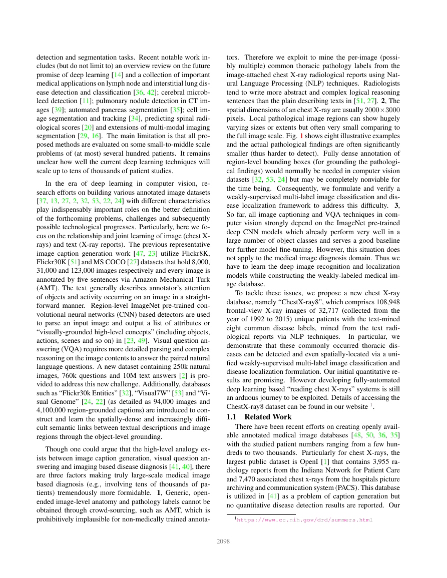As a result, the ChestX-ray8 database is composed of 108,948 frontal-view X-ray images (from 32,717 patients) and each image is la- beled with one or multiple pathology keywords or “Normal” otherwise. Fig. 2 illustrates the correlation of the resulted keywords. It reveals some connections between different pathologies, which agree with radiologists’ domain knowl- edge, e.g., Inﬁltration is often associated with Atelectasis and Effusion. To some extend, this is similar with under- standing the interactions and relationships among objects or concepts in natural images [24]. 2.1 Labeling Disease Names by Text Mining Overall, our approach produces labels using the reports in two passes. In the ﬁrst iteration, we detected all the dis- ease concept in the corpus. The main body of each chest X-ray report is generally structured as “Comparison”, “In- dication”, “Findings”, and “Impression” sections. Here, we focus on detecting disease concepts in the Findings and Im- pression sections. If a report contains neither of these two sections, the full-length report will then be considered. In the second pass, we code the reports as “Normal” if they do not contain any diseases (not limited to 8 predeﬁned pathologies). Pathology Detection: We mine the radiology reports for disease concepts using two tools, DNorm [26] and MetaMap [3]. DNorm is a machine learning method for disease recognition and normalization. It maps every men- tion of keywords in a report to a unique concept ID in the Systematized Nomenclature of Medicine Clinical Terms Figure 2. The circular diagram shows the proportions of images with multi-labels in each of 8 pathology classes and the labels’ co-occurrence statistics. (or SNOMED-CT), which is a standardized vocabulary of clinical terminology for the electronic exchange of clinical health information. tool MetaMap is another prominent to detect bio- concepts from the biomedical text corpus. Different from DNorm, it is an ontology-based approach for the detec- tion of Uniﬁed Medical Language System R (UMLS R) Metathesaurus. In this work, we only consider the seman- tic types of Diseases or Syndromes and Findings (namely ‘dsyn’ and ‘fndg’ respectively). To maximize the recall of our automatic disease detection, we merge the results of DNorm and MetaMap. Table 1 (in the supplemen- tary material) shows the corresponding SNOMED-CT con- cepts that are relevant to the eight target diseases (these mappings are developed by searching the disease names in the UMLS Rterminology service 2, and veriﬁed by a board- certiﬁed radiologist. Negation and Uncertainty: The disease detection algo- rithm locates every keyword mentioned in the radiology re- port no matter if it is truly present or negated. To eliminate the noisy labeling, we need to rule out those negated patho- logical statements and, more importantly, uncertain men- tions of ﬁndings and diseases, e.g., “suggesting obstructive lung disease”. Although many text processing systems (such as [6]) can handle the negation/uncertainty detection problem, most of them exploit regular expressions on the text directly. One of the disadvantages to use regular expressions for nega- tion/uncertainty detection is that they cannot capture vari- 2https://uts.nlm.nih.gov/metathesaurus.html 2099

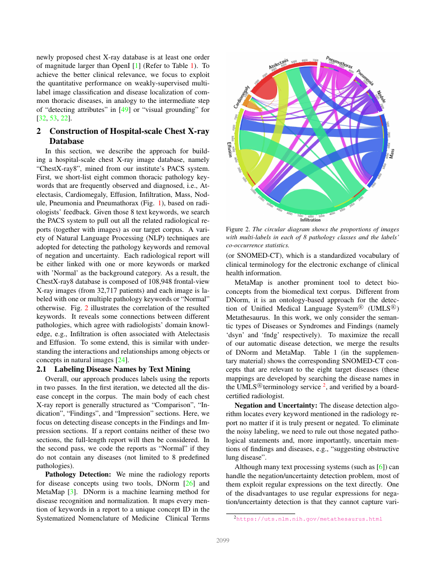
prep of conj or conj or ... clear of focal airspace disease , pneumothorax , or pleural eﬀusion prep of (CCProcessed) prep of (CCProcessed) Figure 3. The dependency graph of text: “clear of focal airspace disease, pneumothorax, or pleural effusion”. ous syntactic constructions for multiple subjects. For exam- ple, in the phrase of “clear of A and B”, the regular expres- sion can capture “A” as a negation but not “B”, particularly when both “A” and “B” are long and complex noun phrases (“clear of focal airspace disease, pneumothorax, or pleural effusion” in Fig. 3). To overcome this complication, we hand-craft a number of novel rules of negation/uncertainty deﬁned on the syn- tactic level in this work. More speciﬁcally, we utilize the syntactic dependency information because it is close to the semantic relationship between words and thus has become prevalent in biomedical text processing. We deﬁned our rules on the dependency graph, by utilizing the dependency label and direction information between words. As the ﬁrst step of preprocessing, we split and tokenize the reports into sentences using NLTK [5]. Next we parse each sentence by the Bllip parser [7] using David Mc- Closkys biomedical model [28]. The syntactic dependen- cies are then obtained from “CCProcessed” dependencies output by applying Stanford dependencies converter [8] on the parse tree. The “CCProcessed” representation propa- gates conjunct dependencies thus simpliﬁes coordinations. As a result, we can use fewer rules to match more com- plex constructions. For an example as shown in Fig. 3, we could use “clear → prep of → DISEASE” to detect three negations from the text hneg, focal airspace diseasei, hneg, pneumothoraxi, and hneg, pleural effusioni. Furthermore, we label a radiology report as “normal” if it meets one of the following criteria: • If there is no disease detected in the report. Note that here we not only consider 8 diseases of interest in this paper, but all diseases detected in the reports. • If the report contains text-mined concepts of “normal” or “normal size” (CUIs C0205307 and C0332506 in the SNOMED-CT concepts respectively). Item # OpenI Ov. ChestX-ray8 Ov. Report Annotations Atelectasis Cardiomegaly Effusion Inﬁltration Mass Nodule Pneumonia Pneumothorax Normal 2,435 2,435 315 345 153 60 15 106 40 22 1,379 - - 122 100 94 45 4 18 15 11 0 108,948 - 5,789 1,010 6,331 10,317 6,046 1,971 1,062 2,793 84,312 - - 3,286 475 4,017 4,698 3,432 1,041 703 1,403 0 Table 1. Total number (#) and # of Overlap (Ov.) of the corpus in both OpenI and ChestX-ray8 datasets. Disease Atelectasis Cardiomegaly Effusion Inﬁltration Mass Nodule Normal Pneumonia Pneumothorax Total MetaMap P / R / F Our Method P / R / F 0.95 / 0.95 / 0.95 0.99 / 0.83 / 0.90 0.74 / 0.90 / 0.81 0.25 / 0.98 / 0.39 0.59 / 0.67 / 0.62 0.95 / 0.65 / 0.77 0.93 / 0.90 / 0.91 0.58 / 0.93 / 0.71 0.32 / 0.82 / 0.46 0.84 / 0.88 / 0.86 0.99 / 0.85 / 0.91 1.00 / 0.79 / 0.88 0.93 / 0.82 / 0.87 0.74 / 0.87 / 0.80 0.75 / 0.40 / 0.52 0.96 / 0.62 / 0.75 0.87 / 0.99 / 0.93 0.66 / 0.93 / 0.77 0.90 / 0.82 / 0.86 0.90 / 0.91 / 0.90 Table 2. Evaluation of image labeling results on OpenI dataset. Performance is reported using P, R, F1-score. the gold standard for evaluating our method. Table 1 sum- marizes the statistics of the subset of OpenI [1, 19] reports. Table 2 shows the results of our method using OpenI, mea- sured in precision (P), recall (R), and F1-score. Higher pre- cision of 0.90, higher recall of 0.91, and higher F1-score of 0.90 are achieved compared to the existing MetaMap ap- proach (with NegEx enabled). For all diseases, our method obtains higher precisions, particularly in “pneumothorax” (0.90 vs. 0.32) and “inﬁltration” (0.74 vs. 0.25). This in- dicates that the usage of negation and uncertainty detection on syntactic level successfully removes false positive cases. More importantly, the higher precisions meet our expecta- tion to generate a Chest X-ray corpus with accurate seman- tic labels, to lay a solid foundation for the later processes. 2.2 Quality Control on Disease Labeling 2.3 Processing Chest X-ray Images To validate our method, we perform the following exper- iments. Given the fact that no gold-standard labels exist for our dataset, we resort to some existing annotated corpora as an alternative. Using the OpenI API [1], we retrieve a total of 3,851 unique radiology reports where each OpenI report is assigned with its key ﬁndings/disease names by human annotators [9]. Given our focus on the eight diseases, a sub- set of OpenI reports and their human annotations are used as Comparing to the popular ImageNet classiﬁcation prob- lem, signiﬁcantly smaller spatial extents of many diseases inside the typical X-ray image dimensions of 3000 × 2000 pixels impose challenges in both the capacity of comput- ing hardware and the design of deep learning paradigm. In ChestX-ray8, X-rays images are directly extracted from the DICOM ﬁle and resized as 1024×1024 bitmap images with- out signiﬁcantly losing the detail contents, compared with 2100

image sizes of 512 × 512 in OpenI dataset. Their intensity ranges are rescaled using the default window settings stored in the DICOM header ﬁles. 2.4 Bounding Box for Pathologies As part of the ChestX-ray8 database, a small number of images with pathology are provided with hand labeled bounding boxes (B-Boxes), which can be used as the ground truth to evaluate the disease localization performance. Fur- thermore, it could also be adopted for one/low-shot learn- ing setup [15], in which only one or several samples are needed to initialize the learning and the system will then evolve by itself with more unlabeled data. We leave this as future work. In our labeling process, we ﬁrst select 200 instances for each pathology (1,600 instances total), consisting of 983 images. Given an image and a disease keyword, a board- certiﬁed radiologist identiﬁed only the corresponding dis- ease instance in the image and labeled it with a B-Box. The B-Box is then outputted as an XML ﬁle. If one image con- tains multiple disease instances, each disease instance is la- beled separately and stored into individual XML ﬁles. As an application of the proposed ChestX-ray8 database and benchmarking, we will demonstrate the detection and local- ization of thoracic diseases in the following. 3 Common Thoracic Disease Detection and Localization Reading and diagnosing Chest X-ray images may be an entry-level task for radiologists but, in fact it is a complex reasoning problem which often requires careful observation and good knowledge of anatomical principles, physiology and pathology. Such factors increase the difﬁculty of de- veloping a consistent and automated technique for reading chest X-ray images while simultaneously considering all common thoracic diseases. As the main application of ChestX-ray8 dataset, we present a uniﬁed weakly-supervised multi-label image clas- siﬁcation and pathology localization framework, which can detect the presence of multiple pathologies and subse- quently generate bounding boxes around the corresponding pathologies. In details, we tailor Deep Convolutional Neural Network (DCNN) architectures for weakly-supervised ob- ject localization, by considering large image capacity, vari- ous multi-label CNN losses and different pooling strategies. 3.1 Uniﬁed DCNN Framework Our goal is to ﬁrst detect if one or multiple pathologies are presented in each X-ray image and later we can lo- cate them using the activation and weights extracted from the network. 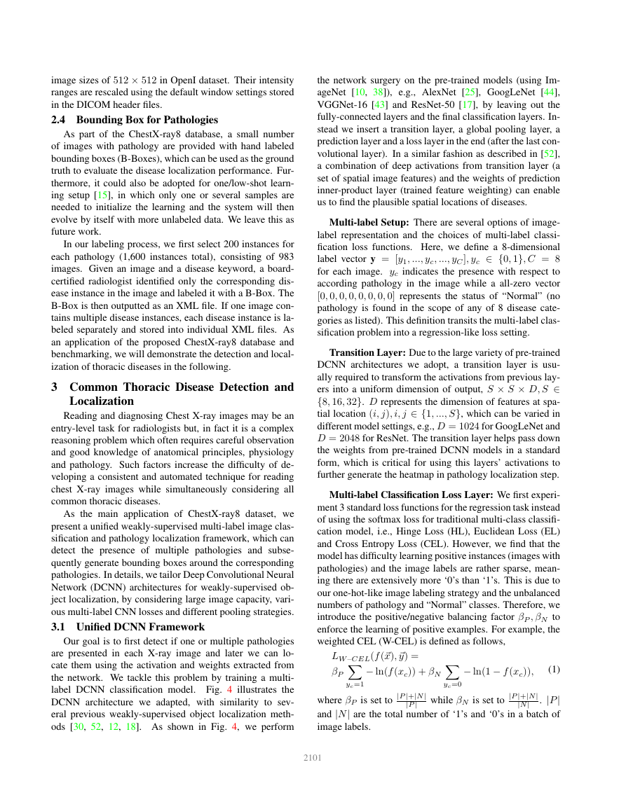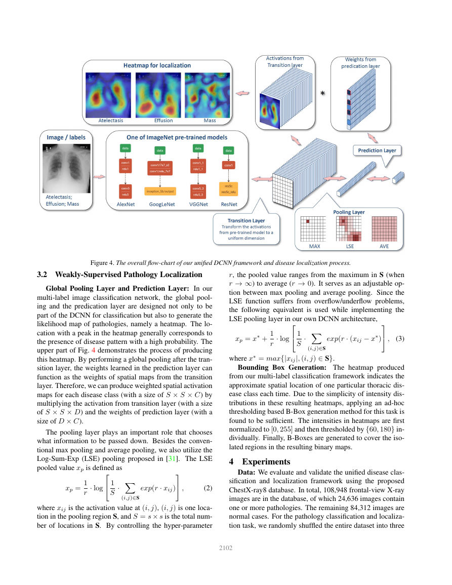We tackle this problem by training a multi- label DCNN classiﬁcation model. Fig. 4 illustrates the DCNN architecture we adapted, with similarity to sev- eral previous weakly-supervised object localization meth- ods [30, 52, 12, 18]. As shown in Fig. 4, we perform the network surgery on the pre-trained models (using Im- ageNet [10, 38]), e.g., AlexNet [25], GoogLeNet [44], VGGNet-16 [43] and ResNet-50 [17], by leaving out the fully-connected layers and the ﬁnal classiﬁcation layers. In- stead we insert a transition layer, a global pooling layer, a prediction layer and a loss layer in the end (after the last con- volutional layer). In a similar fashion as described in [52], a combination of deep activations from transition layer (a set of spatial image features) and the weights of prediction inner-product layer (trained feature weighting) can enable us to ﬁnd the plausible spatial locations of diseases. Multi-label Setup: There are several options of image- label representation and the choices of multi-label classi- ﬁcation loss functions. Here, we deﬁne a 8-dimensional label vector y = [y1, ..., yc, ..., yC], yc ∈ {0, 1}, C = 8 for each image. yc indicates the presence with respect to according pathology in the image while a all-zero vector [0, 0, 0, 0, 0, 0, 0, 0] represents the status of “Normal” (no pathology is found in the scope of any of 8 disease cate- gories as listed). This deﬁnition transits the multi-label clas- siﬁcation problem into a regression-like loss setting. Transition Layer: Due to the large variety of pre-trained DCNN architectures we adopt, a transition layer is usu- ally required to transform the activations from previous lay- ers into a uniform dimension of output, S × S × D, S ∈ {8, 16, 32}. D represents the dimension of features at spa- tial location (i, j), i, j ∈ {1, ..., S}, which can be varied in different model settings, e.g., D = 1024 for GoogLeNet and D = 2048 for ResNet. The transition layer helps pass down the weights from pre-trained DCNN models in a standard form, which is critical for using this layers’ activations to further generate the heatmap in pathology localization step. Multi-label Classiﬁcation Loss Layer: We ﬁrst experi- ment 3 standard loss functions for the regression task instead of using the softmax loss for traditional multi-class classiﬁ- cation model, i.e., Hinge Loss (HL), Euclidean Loss (EL) and Cross Entropy Loss (CEL). However, we ﬁnd that the model has difﬁculty learning positive instances (images with pathologies) and the image labels are rather sparse, mean- ing there are extensively more ‘0’s than ‘1’s. This is due to our one-hot-like image labeling strategy and the unbalanced numbers of pathology and “Normal” classes. Therefore, we introduce the positive/negative balancing factor βP , βN to enforce the learning of positive examples. For example, the weighted CEL (W-CEL) is deﬁned as follows, LW –CEL(f (~x), ~y) = βP X − ln(f (xc)) + βN X yc=1 yc=0 − ln(1 − f (xc)), (1) where βP is set to |P |+|N | . |P | and |N | are the total number of ‘1’s and ‘0’s in a batch of image labels. |P | while βN is set to |P |+|N | |N | 2101

Figure 4. The overall ﬂow-chart of our uniﬁed DCNN framework and disease localization process. 3.2 Weakly-Supervised Pathology Localization Global Pooling Layer and Prediction Layer: In our multi-label image classiﬁcation network, the global pool- ing and the predication layer are designed not only to be part of the DCNN for classiﬁcation but also to generate the likelihood map of pathologies, namely a heatmap. The lo- cation with a peak in the heatmap generally corresponds to the presence of disease pattern with a high probability. The upper part of Fig. 4 demonstrates the process of producing this heatmap. By performing a global pooling after the tran- sition layer, the weights learned in the prediction layer can function as the weights of spatial maps from the transition layer. Therefore, we can produce weighted spatial activation maps for each disease class (with a size of S × S × C) by multiplying the activation from transition layer (with a size of S × S × D) and the weights of prediction layer (with a size of D × C). The pooling layer plays an important role that chooses what information to be passed down. Besides the conven- tional max pooling and average pooling, we also utilize the Log-Sum-Exp (LSE) pooling proposed in [31]. The LSE pooled value xp is deﬁned as xp = 1 r · log   1 S · X (i,j)∈S exp(r · xij)   , (2) where xij is the activation value at (i, j), (i, j) is one loca- tion in the pooling region S, and S = s × s is the total num- ber of locations in S. By controlling the hyper-parameter r, the pooled value ranges from the maximum in S (when r → ∞) to average (r → 0). It serves as an adjustable op- tion between max pooling and average pooling. Since the LSE function suffers from overﬂow/underﬂow problems, the following equivalent is used while implementing the LSE pooling layer in our own DCNN architecture, xp = x∗ + 1 r · log   1 S · X (i,j)∈S exp(r · (xij − x∗)   , (3) where x∗ = max{|xij|, (i, j) ∈ S}. Bounding Box Generation: The heatmap produced from our multi-label classiﬁcation framework indicates the approximate spatial location of one particular thoracic dis- ease class each time. Due to the simplicity of intensity dis- tributions in these resulting heatmaps, applying an ad-hoc thresholding based B-Box generation method for this task is found to be sufﬁcient. The intensities in heatmaps are ﬁrst normalized to [0, 255] and then thresholded by {60, 180} in- dividually. Finally, B-Boxes are generated to cover the iso- lated regions in the resulting binary maps. 4 Experiments Data: We evaluate and validate the uniﬁed disease clas- siﬁcation and localization framework using the proposed ChestX-ray8 database. In total, 108,948 frontal-view X-ray images are in the database, of which 24,636 images contain one or more pathologies. The remaining 84,312 images are normal cases. For the pathology classiﬁcation and localiza- tion task, we randomly shufﬂed the entire dataset into three 2102

subgroups for CNN ﬁne-tuning via Stochastic Gradient De- scent (SGD): i.e. training (70%), validation (10%) and test- ing (20%). We only report the 8 thoracic disease recognition performance on the testing set in our experiments. Further- more, for the 983 images with 1,600 annotated B-Boxes of pathologies, these boxes are only used as the ground truth to evaluate the disease localization accuracy in testing (not for training purpose). CNN Setting: Our multi-label CNN architecture is im- plemented using Caffe framework [21]. The ImageNet pre-trained models, i.e., AlexNet [25], GoogLeNet [44], VGGNet-16 [43] and ResNet-50 [17] are obtained from the Caffe model zoo. Our uniﬁed DCNN takes the weights from those models and only the transition layers and prediction layers are trained from scratch. Due to the large image size and the limit of GPU mem- ory, it is necessary to reduce the image batch size to load the entire model and keep activations in GPU while we in- crease the iter size to accumulate the gradients for more it- erations. The combination of both may vary in different CNN models but we set batch size × iter size = 80 as a constant. Furthermore, the total training iterations are cus- tomized for different CNN models to prevent over-ﬁtting. More complex models like ResNet-50 actually take less it- erations (e.g., 10000 iterations) to reach the convergence. The DCNN models are trained using a Dev-Box linux server with 4 Titan X GPUs. 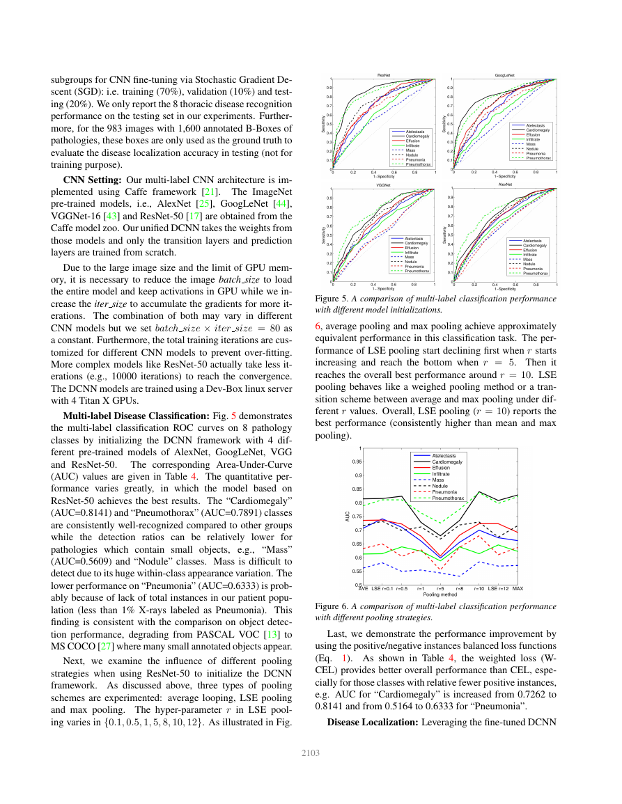Multi-label Disease Classiﬁcation: Fig. 5 demonstrates the multi-label classiﬁcation ROC curves on 8 pathology classes by initializing the DCNN framework with 4 dif- ferent pre-trained models of AlexNet, GoogLeNet, VGG and ResNet-50. The corresponding Area-Under-Curve (AUC) values are given in Table 4. The quantitative per- formance varies greatly, in which the model based on ResNet-50 achieves the best results. The “Cardiomegaly” (AUC=0.8141) and “Pneumothorax” (AUC=0.7891) classes are consistently well-recognized compared to other groups while the detection ratios can be relatively lower for pathologies which contain small objects, e.g., “Mass” (AUC=0.5609) and “Nodule” classes. Mass is difﬁcult to detect due to its huge within-class appearance variation. The lower performance on “Pneumonia” (AUC=0.6333) is prob- ably because of lack of total instances in our patient popu- lation (less than 1% X-rays labeled as Pneumonia). This ﬁnding is consistent with the comparison on object detec- tion performance, degrading from PASCAL VOC [13] to MS COCO [27] where many small annotated objects appear. Next, we examine the inﬂuence of different pooling strategies when using ResNet-50 to initialize the DCNN framework. As discussed above, three types of pooling schemes are experimented: average looping, LSE pooling and max pooling. The hyper-parameter r in LSE pool- ing varies in {0.1, 0.5, 1, 5, 8, 10, 12}. As illustrated in Fig. Figure 5. A comparison of multi-label classiﬁcation performance with different model initializations. 6, average pooling and max pooling achieve approximately equivalent performance in this classiﬁcation task. The per- formance of LSE pooling start declining ﬁrst when r starts increasing and reach the bottom when r = 5. Then it reaches the overall best performance around r = 10. LSE pooling behaves like a weighed pooling method or a tran- sition scheme between average and max pooling under dif- ferent r values. Overall, LSE pooling (r = 10) reports the best performance (consistently higher than mean and max pooling). Figure 6. A comparison of multi-label classiﬁcation performance with different pooling strategies. 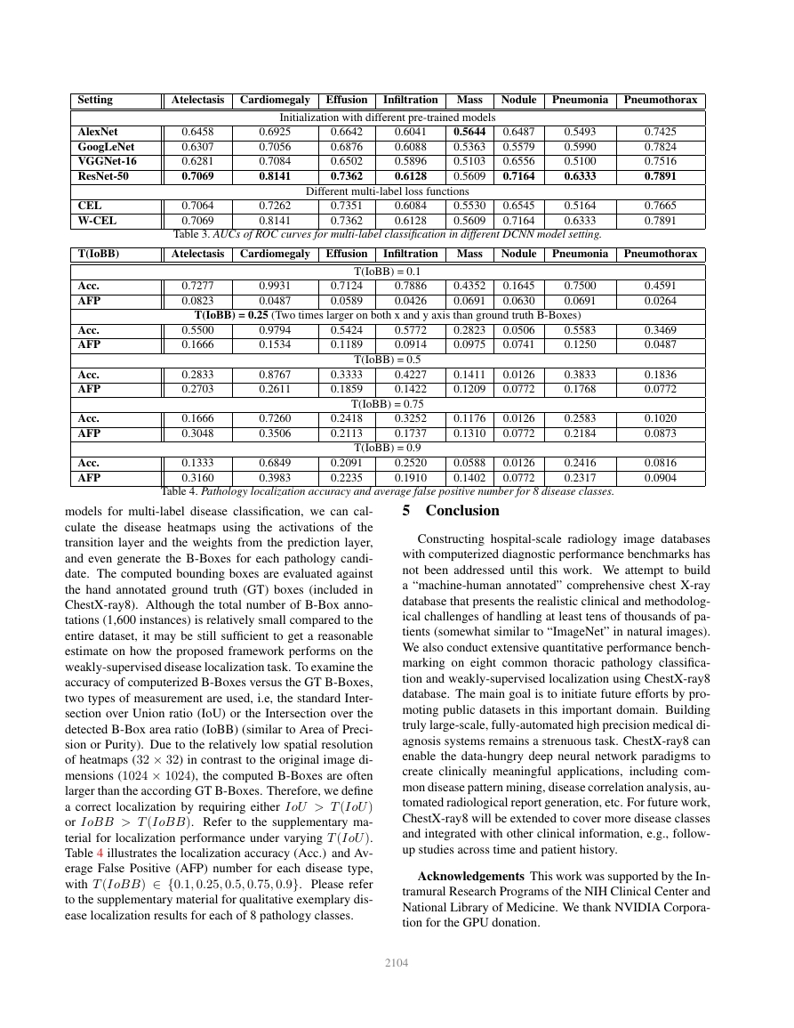Last, we demonstrate the performance improvement by using the positive/negative instances balanced loss functions (Eq. 1). As shown in Table 4, the weighted loss (W- CEL) provides better overall performance than CEL, espe- cially for those classes with relative fewer positive instances, e.g. AUC for “Cardiomegaly” is increased from 0.7262 to 0.8141 and from 0.5164 to 0.6333 for “Pneumonia”. Disease Localization: Leveraging the ﬁne-tuned DCNN 2103

Setting Atelectasis Cardiomegaly Effusion Inﬁltration Mass Nodule Pneumonia Pneumothorax AlexNet GoogLeNet VGGNet-16 ResNet-50 CEL W-CEL 0.6458 0.6307 0.6281 0.7069 0.7064 0.7069 Initialization with different pre-trained models 0.6925 0.7056 0.7084 0.8141 0.7262 0.8141 0.6642 0.6876 0.6502 0.7362 0.6041 0.6088 0.5896 0.6128 0.5644 0.5363 0.5103 0.5609 0.6487 0.5579 0.6556 0.7164 Different multi-label loss functions 0.7351 0.7362 0.6084 0.6128 0.5530 0.5609 0.6545 0.7164 0.5493 0.5990 0.5100 0.6333 0.5164 0.6333 0.7425 0.7824 0.7516 0.7891 0.7665 0.7891 Table 3. AUCs of ROC curves for multi-label classiﬁcation in different DCNN model setting. T(IoBB) Atelectasis Cardiomegaly Effusion Inﬁltration Mass Nodule Pneumonia Pneumothorax Acc. AFP Acc. AFP Acc. AFP Acc. AFP Acc. AFP T(IoBB) = 0.1 0.7277 0.0823 0.9931 0.0487 0.7124 0.0589 0.7886 0.0426 0.4352 0.0691 0.1645 0.0630 0.7500 0.0691 T(IoBB) = 0.25 (Two times larger on both x and y axis than ground truth B-Boxes) 0.5500 0.1666 0.2833 0.2703 0.1666 0.3048 0.1333 0.3160 0.9794 0.1534 0.8767 0.2611 0.7260 0.3506 0.6849 0.3983 0.5424 0.1189 0.5772 0.0914 0.2823 0.0975 0.0506 0.0741 T(IoBB) = 0.5 0.3333 0.1859 0.2418 0.2113 0.4227 0.1422 T(IoBB) = 0.75 0.3252 0.1737 0.1411 0.1209 0.0126 0.0772 0.1176 0.1310 0.0126 0.0772 T(IoBB) = 0.9 0.2091 0.2235 0.2520 0.1910 0.0588 0.1402 0.0126 0.0772 0.5583 0.1250 0.3833 0.1768 0.2583 0.2184 0.2416 0.2317 0.4591 0.0264 0.3469 0.0487 0.1836 0.0772 0.1020 0.0873 0.0816 0.0904 Table 4. Pathology localization accuracy and average false positive number for 8 disease classes. models for multi-label disease classiﬁcation, we can cal- culate the disease heatmaps using the activations of the transition layer and the weights from the prediction layer, and even generate the B-Boxes for each pathology candi- date. The computed bounding boxes are evaluated against the hand annotated ground truth (GT) boxes (included in ChestX-ray8). Although the total number of B-Box anno- tations (1,600 instances) is relatively small compared to the entire dataset, it may be still sufﬁcient to get a reasonable estimate on how the proposed framework performs on the weakly-supervised disease localization task. To examine the accuracy of computerized B-Boxes versus the GT B-Boxes, two types of measurement are used, i.e, the standard Inter- section over Union ratio (IoU) or the Intersection over the detected B-Box area ratio (IoBB) (similar to Area of Preci- sion or Purity). Due to the relatively low spatial resolution of heatmaps (32 × 32) in contrast to the original image di- mensions (1024 × 1024), the computed B-Boxes are often larger than the according GT B-Boxes. Therefore, we deﬁne a correct localization by requiring either IoU > T (IoU ) or IoBB > T (IoBB). Refer to the supplementary ma- terial for localization performance under varying T (IoU ). Table 4 illustrates the localization accuracy (Acc.) and Av- erage False Positive (AFP) number for each disease type, with T (IoBB) ∈ {0.1, 0.25, 0.5, 0.75, 0.9}. Please refer to the supplementary material for qualitative exemplary dis- ease localization results for each of 8 pathology classes. 5 Conclusion Constructing hospital-scale radiology image databases with computerized diagnostic performance benchmarks has not been addressed until this work. We attempt to build a “machine-human annotated” comprehensive chest X-ray database that presents the realistic clinical and methodolog- ical challenges of handling at least tens of thousands of pa- tients (somewhat similar to “ImageNet” in natural images). We also conduct extensive quantitative performance bench- marking on eight common thoracic pathology classiﬁca- tion and weakly-supervised localization using ChestX-ray8 database. The main goal is to initiate future efforts by pro- moting public datasets in this important domain. Building truly large-scale, fully-automated high precision medical di- agnosis systems remains a strenuous task. ChestX-ray8 can enable the data-hungry deep neural network paradigms to create clinically meaningful applications, including com- mon disease pattern mining, disease correlation analysis, au- tomated radiological report generation, etc. For future work, ChestX-ray8 will be extended to cover more disease classes and integrated with other clinical information, e.g., follow- up studies across time and patient history. Acknowledgements This work was supported by the In- tramural Research Programs of the NIH Clinical Center and National Library of Medicine. We thank NVIDIA Corpora- tion for the GPU donation. 2104

分享到：

赞收藏

资料库

Wang_ChestX-ray8_Hospital-Scale_Chest_CVPR_2017_paper.pdf

相关推荐

人工智能

热门标签

最新资料