gCLUTO – An Interactive Clustering, Visualization, and
Analysis System ∗
Matt Rasmussen
University of Minnesota, Department of
Computer Science and Engineering
Minneapolis, MN 55455
mrasmus@cs.umn.edu
ABSTRACT
Clustering algorithms are exploratory data analysis tools that have
proved to be essential for gaining valuable insights on various as-
pects and relationships of the underlying systems. In this paper we
present gCLUTO, a stand-alone clustering software package which
serves as an easy-to-use platform that combines clustering algo-
rithms along with a number of analysis, reporting, and visualization
tools to aid in interactive exploration and clustering-driven analysis
of large datasets. gCLUTO provides a wide-range of algorithms that
operate either directly on the original feature-based representation
of the objects or on the object-to-object similarity graphs and are
capable of analyzing different types of datasets and finding clusters
with different characteristics. In addition, gCLUTO implements a
project-oriented work-flow that eases the process of data analysis.
Keywords
Cluster analysis, interactive data exploration, information visual-
ization
INTRODUCTION
1.
Due to recent advances in information technology, there has been
an enormous growth in the amount of data generated in fields rang-
ing from business to the sciences. This data has the potential to
greatly benefit its owners by increasing their understanding of their
own work. However, the growing size and complexity of data has
∗This work was supported in part by NSF CCR-9972519, EIA-
9986042, ACI-9982274, ACI-0133464, and ACI-0312828;
the
Digital Technology Center at the University of Minnesota; and
by the Army High Performance Computing Research Center (AH-
PCRC) under the auspices of the Department of the Army, Army
Research Laboratory (ARL) under Cooperative Agreement number
DAAD19-01-2-0014. The content of which does not necessarily
reflect the position or the policy of the government, and no official
endorsement should be inferred. Access to research and computing
facilities was provided by the Digital Technology Center and the
Minnesota Supercomputing Institute.
CSE/UMN Technical Report: TR# 04–021
George Karypis
University of Minnesota, Department of
Computer Science and Engineering,
Digital Technology Center, and Army HPC
Research Center, Minneapolis, MN 55455
karypis@cs.umn.edu
introduced new challenges in analyzing and extracting its mean-
ing. As a result, data mining methods, which employ a variety of
computational techniques are becoming increasingly important as
the only viable approach to efficiently and effectively extract new
information from these large datasets.
One technique in particular, clustering, has been successful in a
wide range of knowledge discovery applications. Clustering is an
exploratory data analysis process [47, 7] that groups a set of data
items such that the intra-cluster similarity is maximized and the
inter-cluster similarity is minimized. These discovered clusters can
be used to explain the characteristics of the underlying data dis-
tribution, provide insights on various aspects and relationships of
the underlying systems, and serve as the foundation for other data
mining and analysis tasks.
The topic of clustering has been extensively studied in many scien-
tific disciplines and over the years a variety of different algorithms
have been developed [32, 6, 26, 20, 35, 4, 53, 6, 12, 52, 15, 16,
23, 9, 25]. Two relatively recent surveys on the topics [21, 17]
offer a comprehensive summary of the different applications and
algorithms. This work provides a wide variety of techniques that
are suited for clustering different types of datasets and find clusters
that satisfy different properties.
However, along with increasing choices for algorithms and param-
eters has come increasing complexity of the data analysis process.
Without proper selection of a clustering algorithm or parameters,
important structures within the data may be overlooked. Therefore,
there exists a need for a clustering analysis work bench, a single
interactive work space where many clustering algorithms, visual-
izations, and analysis tools are available to use in a way that allows
the user to efficiently explore the best method of analyzing their
data.
In this paper, we introduce gCLUTO, a stand alone clustering soft-
ware package designed to ease the use of clustering algorithms and
their results. gCLUTO offers improvements over existing tools by
providing features that make clustering practical for a wide vari-
ety of applications. First, gCLUTO provides an array of clustering
algorithms and options through the use of the CLUTO clustering
library [25]. The CLUTO library provides highly optimized imple-
mentations of agglomerative, k-means, and graph clustering, es-
pecially in the context of sparse high-dimensional data. Second,
gCLUTO helps the user sort through the algorithm options and re-
sulting data files by providing a intuitive graphical interface. Fol-
�
lowing the paradigm of most development tools, gCLUTO uses
the concept of a “project” in order to organize the user’s various
datasets, clustering solutions, and visualizations. Third, gCLUTO
provides both standard statistics and unique visualizations for in-
terpreting clustering results. Given the wide range of options and
factors that are involved in clustering, the user should carefully an-
alyze their results and compare them with results generated with
differing options. Therefore, additional effort has gone into visu-
alizations that can facilitate analysis and comparisons. Lastly, the
software package has been designed to suit a wide range of users
from different problem domains who may or may not be knowl-
edgeable about the subtleties of clustering. Accordingly, reason-
able defaults are available for users who want quick results, while
power users have access to all configuration options involved in
clustering. Most importantly, these options and analysis tools are
tightly integrated into a single interactive work bench that can serve
as the user’s main work space for carrying out analysis.
The rest of this paper is organized as follows. Section 2 describes
some of the existing work that is most closely related to the topic of
this paper. Section 3 provides a detailed description of gCLUTO by
briefly describing the various clustering algorithms that it incorpo-
rates, its project-oriented work-flow, and its various visualization,
and analysis capabilities. Finally, Section 4 provides some con-
cluding remarks and describes our ongoing and future efforts on
enhancing its capabilities and applications.
2. RELATED WORK
There are a number of commercial tools that integrate clustering
methods in an easy-to-use graphical and interactive environment.
Many of these tools, which include SAS’s enterprise miner, SPSS’s
Clementine, and IBM’s Intelligent miner, are available within the
context of a larger application suite focusing on providing an in-
tegrated environment for data mining and analysis. Even though
these tools are highly integrated, have advanced data import/export
capabilities, and provide a variety of information visualization tech-
niques, they tend to provide only a small number of different clus-
tering algorithms limiting both the types of analysis that can be
performed and the types of datasets that can be analyzed.
In recent years, within the context of research in the life sciences,
cluster analysis has emerged as an essential tool for analyzing gene
expression datasets derived from microarrays and DNA chips [13,
50, 41, 55]. This has led to the development of a number of com-
mercial and publicly available integrated tools for performing clus-
ter analysis on this type of datasets. Among these are SpotFire
Decision Site [46], the Rosetta Resolver [37], Expressionist [14],
Cluster and TreeView [11], GeneCluster [5], BioConductor [10],
TM4 [38], as well as others. Most of these tools are highly so-
phisticated, offer a variety of different clustering algorithms, and
have extensive visualization capabilities. However, since they are
designed to analyze gene expression datasets, they can only oper-
ate on datasets whose objects are represented with relatively low-
dimensional dense feature vectors and cannot operate (or scale) to
large, high-dimensional sparse datasets (e.g., datasets derived from
customer transactions or document datasets).
lection and to that extent they provide a number of sophisticated
visualizations that help the user to quickly focus on the informa-
tion that he or she wants. However, they are not designed to be
general purpose cluster analysis tools, as they only include a small
number of different clustering algorithms and they are focused on
a specific task.
Finally, a number of different techniques have been developed for
visualizing clustering solutions. This research falls within the broad
area of information visualization and its goal is to provide the user
with an intuitive representation of the underlying dataset by show-
ing/highlighting the inter- and intra-relationships between the ob-
jects across and within clusters. Examples of such techniques in-
clude various 2D and 3D dendrograms [43, 19], which are highly
effective for representing hierarchical clustering solutions; 2D and
3D non-linear projections of clustering solutions such as Sammon
map [40], MDS [30], SOM [29], and various projections based on
PCA and LSI [20, 4]; and hyperbolic visualizations [31, 19, 51].
3. gCLUTO: INTERACTIVE CLUSTERING,
VISUALIZATION, AND ANALYSIS
gCLUTO’s primary design goals are to provide an easy-to-use plat-
form that combines a variety of different clustering algorithms,
which are capable of analyzing different types of datasets and find-
ing clusters with different characteristics, along with a number of
analysis, reporting, and visualization tools to aid in the interactive
exploration and clustering-driven analysis of large datasets. To-
ward these goals, gCLUTO provides a wide-range of clustering al-
gorithms that operate either directly on the original feature-based
representation of the objects or on the object-to-object similarity
graphs and a project-oriented work-flow that eases the process of
data analysis.
3.1 Clustering Algorithms
gCLUTO supports agglomerative, partitional, and graph partitional
clustering algorithms, each of which have different advantages and
disadvantages, are suited for datasets with different characteristics,
and can be used to perform different types of analysis. In addition,
each of these algorithms can be used within the context of a boot-
strap clustering process that uses statistical techniques to determine
the stability of the resulting clustering solutions.
3.1.1 Agglomerative Clustering
Agglomerative algorithms find the clusters by initially assigning
each object to its own cluster and then repeatedly merging pairs of
clusters until either the desired number of clusters has been ob-
tained or all the objects have been merged into a single cluster
leading to a complete agglomerative tree. The key step in these
algorithms is the method used to identify the pairs of clusters to
be merged next. gCLUTO supports ten different merging schemes.
The first three are based on the classical single-link [45], complete-
link [28], and group average [22] approaches, whereas the other
seven, called I1, I2, E1, H1, H2, G1, and G2, are based on some
recently introduced schemes that were motivated by research on
partitional clustering [54].
There are a number of different systems that are specifically de-
signed for the interactive exploration/visualization of document col-
lections and query results that use document clustering and clus-
ter visualization as one of the mechanisms to facilitate this type
of analysis [3, 18, 8, 33, 49, 42, 34]. The primary goal of these
systems is to aid the user in navigating through the document col-
These schemes differ on how the similarity between the individual
objects in the various clusters are combined to determine the sim-
ilarity between the clusters themselves. The single-link criterion
function measures the similarity of two clusters by the maximum
similarity between any pair of objects from each cluster, whereas
the complete-link uses the minimum similarity. In general, both
�
the single- and the complete-link approaches do not work very well
because they either base their decisions to a limited amount of in-
formation (single-link), or assume that all the objects in the cluster
are very similar to each other (complete-link). On the other hand,
the group average approach measures the similarity of two clusters
by the average of the pairwise similarity of the objects from each
cluster and does not suffer from the problems arising with single-
and complete-link. The remaining seven schemes take an entirely
different approach and treat the clustering process as an optimiza-
tion problem by selecting the cluster-pairs that optimize various as-
pects of intra-cluster similarity, inter-cluster dissimilarity, and their
combinations. The advantage of these schemes is that they lead
to more natural clusters and agglomerative trees that are more bal-
anced than the more traditional schemes. A precise description of
these schemes is beyond the scope of this paper, and the reader
should refer to [54, 56] for a detailed description and comparative
evaluation.
3.1.2 Partitional Clustering
Partitional clustering algorithms find the clusters by partitioning the
entire dataset into a predetermined number of disjoint sets, each
corresponding to a single cluster. This partitioning is achieved by
treating the clustering process as an optimization procedure that
tries to create high quality clusters according to a particular func-
tion that reflects the underlying definition of the “goodness” of the
clusters. This function is referred to as the clustering criterion func-
tion and gCLUTO implements seven such criterion functions (that
are similar to the I1, I2, E1, H1, H2, G1, and G2 schemes used by
agglomerative clustering) and have been shown to produce high-
quality clusters in low- and high-dimensional datasets [56].
gCLUTO uses two different methods for computing the partitioning
clustering solution. The first method computes a k-way clustering
solution via a sequence of repeated bisections, whereas the sec-
ond method computes the solution directly (in a fashion similar to
traditional K-means-based algorithms). These methods are often
referred to as repeated bisecting and direct k-way clustering, re-
spectively. In both cases, the clustering solution is computed using
a randomized incremental optimization algorithm that is greedy in
nature, has low computational requirements, and produces high-
quality solutions [56].
3.1.3 Graph Partitional
gCLUTO’s graph-partitioning-based clustering algorithms use a sparse
graph to model the affinity relations between the different objects,
and then discover the desired clusters by partitioning this graph
[23]. To some extent, this approach is similar in spirit with that used
by the partitional clustering algorithms described earlier; however,
unlike those algorithms, the graph-partitioning-based approaches
consider only the affinity relations between an object and a small
number of its most similar other objects. As will be discussed later,
this enables them to find clusters that have inherently different char-
acteristics than those discovered by partitional methods.
gCLUTO provides different methods for constructing this affinity
graph and various post-processing schemes that are designed to
help in identifying the natural clusters in the dataset. The actual
graph partitioning is computed using an efficient multilevel graph-
partitioning algorithm [24] that leads to high-quality partitionings
and clustering solutions.
3.1.4 Bootstrap Clustering
Although the clustering problem is a well-defined optimization prob-
lem, there can still be uncertainty associated with its result due to
uncertainties in the input data. For example, in the case of clus-
tering data generated from measurements, each measurement will
have a margin of error. Without additional analysis, a clustering
algorithm will cluster the data under the assumption that the data
is completely accurate. However, it would be more appropriate if
the algorithm could incorporate the uncertainties associated with
the data to produce a clustering result that could portray its level of
statistical significance given the uncertainties.
Bootstrap clustering is a technique introduced by [27] that adds
the statistical technique of bootstrapping to clustering algorithms.
Bootstrapping simulates the multiple sampling of a distribution by
randomly selecting values from a known sample with replacement.
By sampling with replacement, new hypothetical datasets can be
produced from the original dataset that exhibit the same distribution
of values and uncertainties. This allows clustering algorithms to
explore what results would occur if the same measurements were
taken again.
gCLUTO implements two methods of bootstrapping data: resam-
pling features and resampling residuals. To resample the features
of a dataset, gCLUTO randomly selects with replacement columns
from the dataset to produce a new set of features. This resampling
tests to what extent the clustering algorithm may be relying on any
particular feature. The resampling of residuals is performed by first
supplying a residual matrix for the dataset. A residual matrix con-
tains the errors associated with a dataset, which can be found by
fitting the data to a linear model. In [27], residuals for microarray
data are found by fitting the data to an ANOVA model. gCLUTO
can accept residual matrices stored in character delimited file for-
mats. With the residual matrix, gCLUTO performs bootstrapping to
generate a new residual matrix, which is then added to the original
dataset to produce a new hypothetical dataset.
Bootstrap clustering uses these hypothetical datasets to estimate the
significance of a clustering solution by clustering each hypotheti-
cal dataset and comparing all of their clustering solutions. gCLUTO
provides three statistics for reporting a clustering solution’s signifi-
cance: solution stability, cluster stability, and object stability [36].
The term stability refers to the level of consistency observed be-
tween the various clustering results. These stability measurements
range from zero (no consistency between solutions) to one (com-
plete consistency between solutions). Solution stability represents
the significance of the solution as a whole, where as cluster and
object stability portray a significance level on a per cluster and per
object basis.
gCLUTO compares the various solutions generated by bootstrap
clustering by computing a consensus solution to which a mapping
is found to all other solutions. This star-like mapping arrangement
allows comparisons to be made between any pair of solutions while
also requiring the fewest mappings to be found. The consensus so-
lution is found by generating a solution that is most similar to most
of the solutions. This is done by clustering the objects using a sim-
ilarity graph built from information about the multiple bootstrap
solutions. gCLUTO builds a similarity graph by defining the sim-
ilarity of two objects as the percentage of bootstrap solutions that
assign the two objects to the same cluster. The consensus solution
is also the final solution that gCLUTO presents to the user in the
solution report.
�
3.1.5 Characteristics of the Various Clustering Al-
gorithms
The various clustering algorithms provided by gCLUTO have been
designed, and are well-suited, for finding different types of clusters—
allowing for different types of analysis. There are two general types
of clusters that often arise in different application domains and dif-
ferent analysis requirements. What differentiates them is the simi-
larity relations among the objects assigned to the various clusters.
The first type contains clusters in which the similarity between all
pairs of objects assigned to the same cluster will be high. On the
other hand, the second type contains clusters in which the direct
pairwise similarity between the various objects of the same clus-
ter may be quite low, but within each cluster there exist a suf-
ficiently large number of other objects that eventually “connect”
these low similarity objects. That is, if we consider the object-
to-object similarity graph, then these objects will be connected by
many paths that stay within the cluster that traverse high similarity
edges. The names of these two cluster types have been inspired
by this similarity-based view, and they are referred to as globular
and transitive clusters, respectively. gCLUTO’s partitional and ag-
glomerative algorithms are able to find clusters that are primarily
globular, whereas its graph-partitioning and some of its agglomer-
ative algorithms (e.g., single-link) are capable of finding transitive
clusters.
3.1.6 Similarity Measures
gCLUTO’s feature-based clustering algorithms treat the objects to
be clustered as vectors in a multi-dimensional space and measure
the degree of similarity between these objects using either the co-
sine function, the Pearson’s correlation coefficient, extended Jac-
card coefficient [48], or a similarity measure derived from the Eu-
clidean distance of these vectors. The first two similarity measures
can be used by all clustering algorithms, whereas the last two can
be used only by the graph-partitioning-based algorithms.
By using the cosine and correlation coefficient measures, two ob-
jects are similar if their corresponding vectors1 point in the same
direction (i.e., they have roughly the same set of features and in the
same proportion), regardless of their actual length. On the other
hand, the Euclidean distance does take into account both direction
and magnitude. Finally, similarity based on extended Jaccard co-
efficient accounts both for angle as well as magnitude. These are
some of the most widely used measures, and have been used exten-
sively to cluster a variety of different datasets.
3.1.7 Computational Requirements
gCLUTO’s algorithms have been optimized for operating on very
large datasets both in terms of the number of objects as well as the
number of dimensions. Nevertheless, the various clustering algo-
rithms have different memory and computational scalability char-
acteristics. The agglomerative based schemes can cluster datasets
containing 2,000–5,000 objects in under a minute but due to their
memory requirements they should not be used to cluster datasets
with over 10,000 objects. The partitional algorithms are very scal-
able both in terms of memory and computational complexity, and
can cluster datasets containing several tens of thousands of ob-
jects in a few minutes. Finally, the complexity of the graph-based
schemes is usually between that of agglomerative and partitional
1In the case of Pearson’s correlation coefficient, the vectors are
obtained by first subtracting their average value.
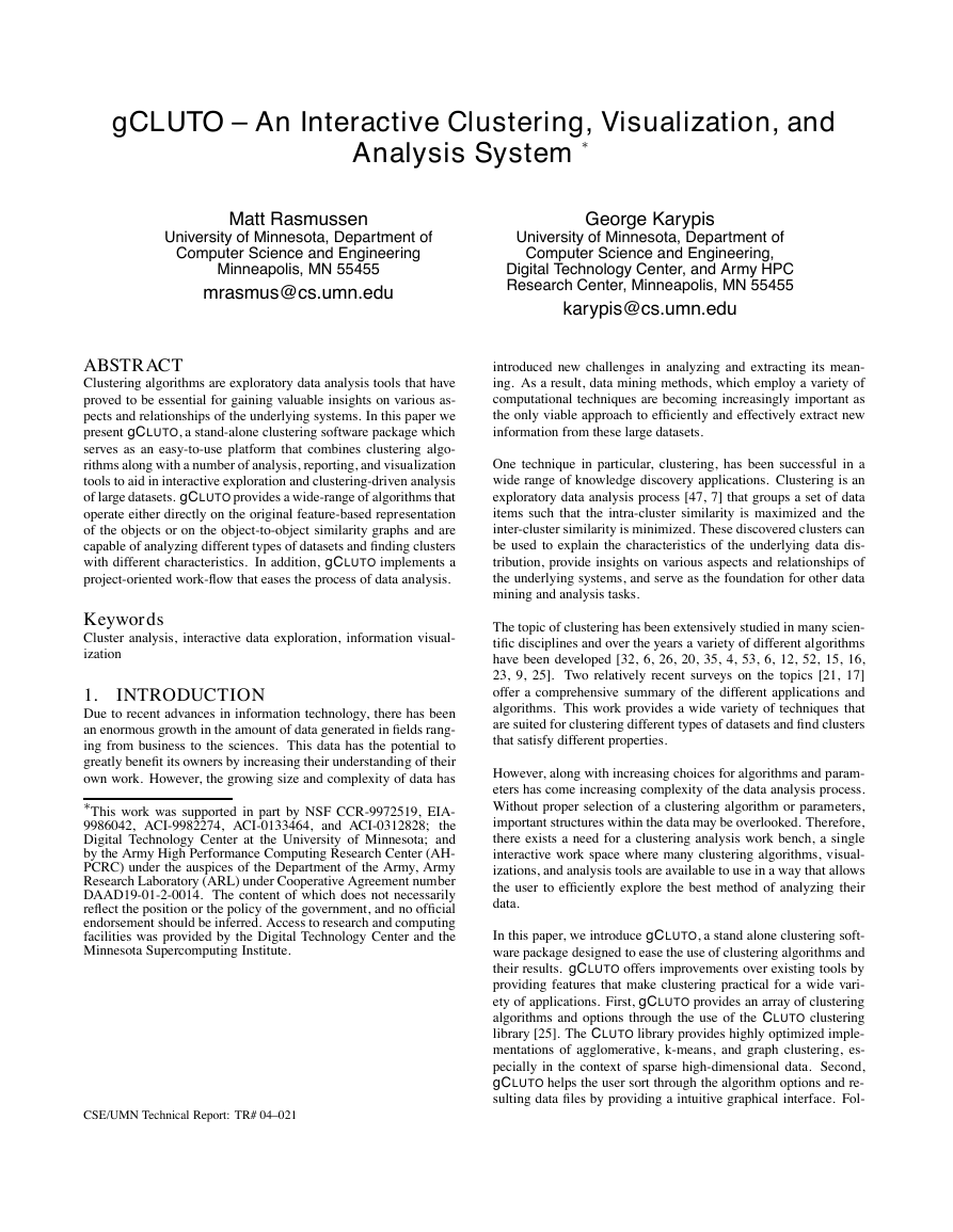
Figure 1: Overview of gCLUTO’s work-flow with example
screen-shots for each stage.
methods and maintain the low memory requirements of the parti-
tional schemes.
3.2 Clustering Work-flow and Organization
The main strength of gCLUTO is its ability to organize the user’s
data and work-flow in a way that eases the process of data anal-
ysis. This work-flow often consists of a sequence of stages, such
as importing and preparing data, selecting clustering options, inter-
preting solution reports, and concluding with visualization. Each
stage of the process demands decisions to be made by the user that
can alter the course of data analysis. Consequently, the user may
want to backtrack to previous stages and create a new branch of
analysis. An overview of this work-flow with examples of branch-
ing is depicted in Figure 1.
gCLUTO assists these types of work-flows by introducing the con-
cept of a project. A project manages the various data files, solu-
tions reports, and visualizations that the user generates by storing
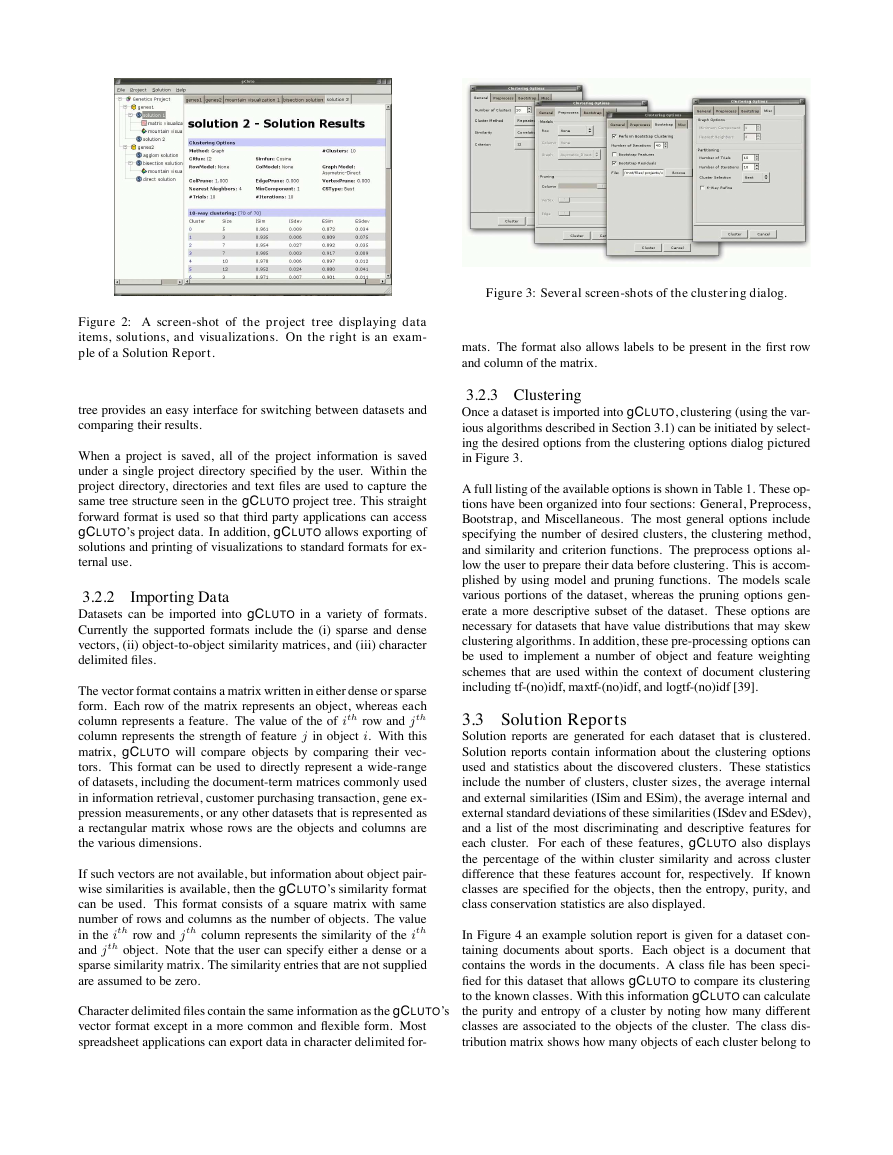
and presenting them in a single container. Figure 2 illustrates how
gCLUTO uses a tree to represent a project as it progresses through
the stages of data analysis.
The work-flow of a user begins by creating a new project. gCLUTO
will create a new directory to hold all project related files as well
as a new empty project tree. Next the user imports one or more re-
lated datasets. These datasets are represented by icons that appear
directly beneath the project tree’s root. After importation, the user
can cluster a dataset to produce a clustering solution. For each so-
lution, a solution report is generated which contains statistics about
the clustering. Clustering solutions are presented by an ‘S’ icon and
are placed beneath the clustered dataset’s icon in the project tree.
As more clustering solutions are generated, the project tree will
continue to organize them by their corresponding datasets. Lastly,
the work-flow concludes with interpreting a solution using one or
more visualizations. Again, the project tree will reflect which solu-
tions have generated visualizations by placing beneath them visu-
alization icons.
3.2.1 Creating a New Project
The user begins their analysis by first creating a new project. A
project is intended to hold one or more related datasets. The project
�
Figure 2: A screen-shot of the project tree displaying data
items, solutions, and visualizations. On the right is an exam-
ple of a Solution Report.
tree provides an easy interface for switching between datasets and
comparing their results.
When a project is saved, all of the project information is saved
under a single project directory specified by the user. Within the
project directory, directories and text files are used to capture the
same tree structure seen in the gCLUTO project tree. This straight
forward format is used so that third party applications can access
gCLUTO’s project data. In addition, gCLUTO allows exporting of
solutions and printing of visualizations to standard formats for ex-
ternal use.
3.2.2 Importing Data
Datasets can be imported into gCLUTO in a variety of formats.
Currently the supported formats include the (i) sparse and dense
vectors, (ii) object-to-object similarity matrices, and (iii) character
delimited files.
The vector format contains a matrix written in either dense or sparse
form. Each row of the matrix represents an object, whereas each
column represents a feature. The value of the of ith row and jth
column represents the strength of feature j in object i. With this
matrix, gCLUTO will compare objects by comparing their vec-
tors. This format can be used to directly represent a wide-range
of datasets, including the document-term matrices commonly used
in information retrieval, customer purchasing transaction, gene ex-
pression measurements, or any other datasets that is represented as
a rectangular matrix whose rows are the objects and columns are
the various dimensions.
If such vectors are not available, but information about object pair-
wise similarities is available, then the gCLUTO’s similarity format
can be used. This format consists of a square matrix with same
number of rows and columns as the number of objects. The value
in the ith row and jth column represents the similarity of the ith
and jth object. Note that the user can specify either a dense or a
sparse similarity matrix. The similarity entries that are not supplied
are assumed to be zero.
Character delimited files contain the same information as the gCLUTO’s
vector format except in a more common and flexible form. Most
spreadsheet applications can export data in character delimited for-
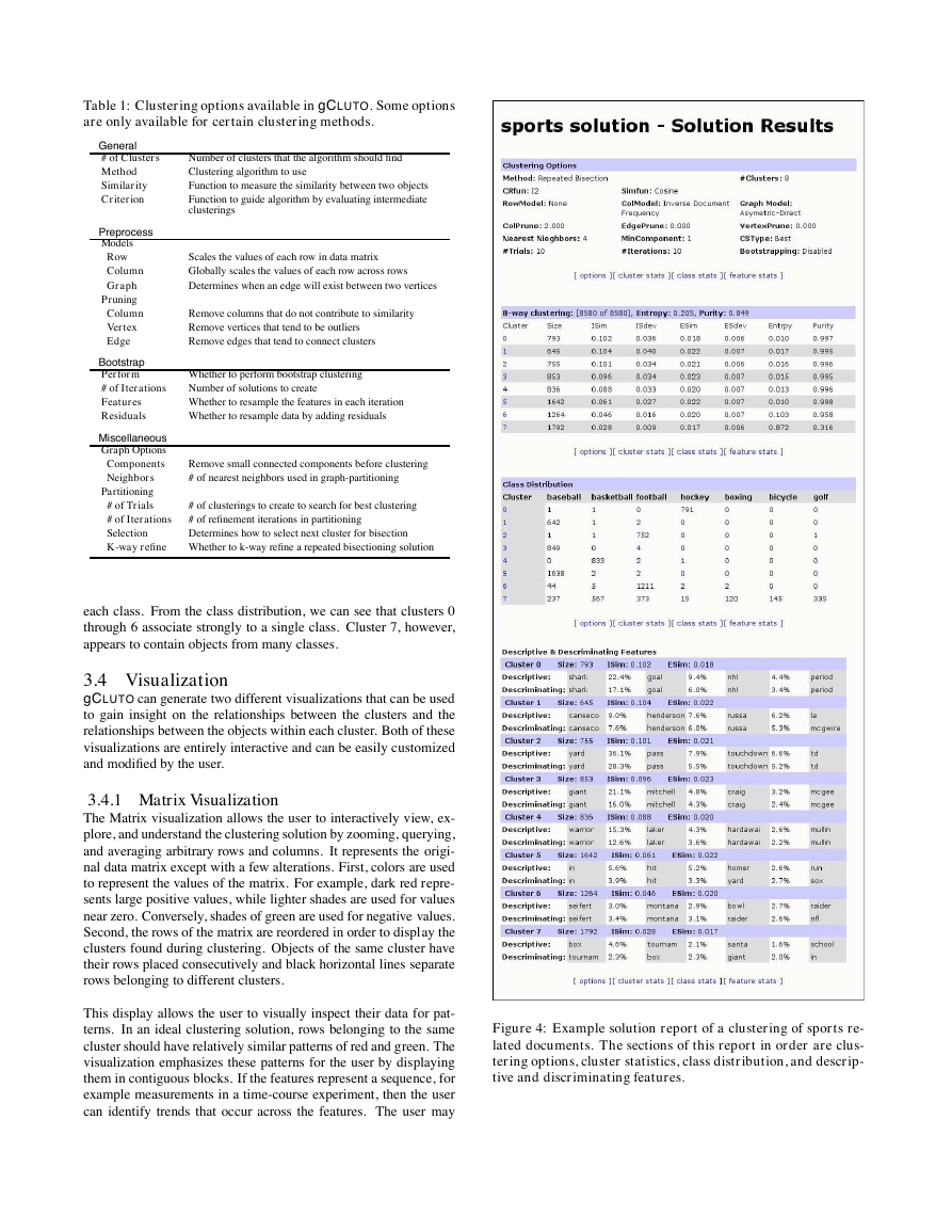
Figure 3: Several screen-shots of the clustering dialog.
mats. The format also allows labels to be present in the first row
and column of the matrix.
3.2.3 Clustering
Once a dataset is imported into gCLUTO, clustering (using the var-
ious algorithms described in Section 3.1) can be initiated by select-
ing the desired options from the clustering options dialog pictured
in Figure 3.
A full listing of the available options is shown in Table 1. These op-
tions have been organized into four sections: General, Preprocess,
Bootstrap, and Miscellaneous. The most general options include
specifying the number of desired clusters, the clustering method,
and similarity and criterion functions. The preprocess options al-
low the user to prepare their data before clustering. This is accom-
plished by using model and pruning functions. The models scale
various portions of the dataset, whereas the pruning options gen-
erate a more descriptive subset of the dataset. These options are
necessary for datasets that have value distributions that may skew
clustering algorithms. In addition, these pre-processing options can
be used to implement a number of object and feature weighting
schemes that are used within the context of document clustering
including tf-(no)idf, maxtf-(no)idf, and logtf-(no)idf [39].
3.3 Solution Reports
Solution reports are generated for each dataset that is clustered.
Solution reports contain information about the clustering options
used and statistics about the discovered clusters. These statistics
include the number of clusters, cluster sizes, the average internal
and external similarities (ISim and ESim), the average internal and
external standard deviations of these similarities (ISdev and ESdev),
and a list of the most discriminating and descriptive features for
each cluster. For each of these features, gCLUTO also displays
the percentage of the within cluster similarity and across cluster
difference that these features account for, respectively. If known
classes are specified for the objects, then the entropy, purity, and
class conservation statistics are also displayed.
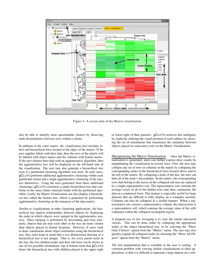
In Figure 4 an example solution report is given for a dataset con-
taining documents about sports. Each object is a document that
contains the words in the documents. A class file has been speci-
fied for this dataset that allows gCLUTO to compare its clustering
to the known classes. With this information gCLUTO can calculate
the purity and entropy of a cluster by noting how many different
classes are associated to the objects of the cluster. The class dis-
tribution matrix shows how many objects of each cluster belong to
�
Table 1: Clustering options available in gCLUTO. Some options
are only available for certain clustering methods.
General
# of Clusters
Method
Similarity
Criterion
Preprocess
Models
Row
Column
Graph
Pruning
Column
Vertex
Edge
Bootstrap
Perform
# of Iterations
Features
Residuals
Miscellaneous
Graph Options
Components
Neighbors
Partitioning
# of Trials
# of Iterations
Selection
K-way refine
Number of clusters that the algorithm should find
Clustering algorithm to use
Function to measure the similarity between two objects
Function to guide algorithm by evaluating intermediate
clusterings
Scales the values of each row in data matrix
Globally scales the values of each row across rows
Determines when an edge will exist between two vertices
Remove columns that do not contribute to similarity
Remove vertices that tend to be outliers
Remove edges that tend to connect clusters
Whether to perform bootstrap clustering
Number of solutions to create
Whether to resample the features in each iteration
Whether to resample data by adding residuals
Remove small connected components before clustering
# of nearest neighbors used in graph-partitioning
# of clusterings to create to search for best clustering
# of refinement iterations in partitioning
Determines how to select next cluster for bisection
Whether to k-way refine a repeated bisectioning solution
each class. From the class distribution, we can see that clusters 0
through 6 associate strongly to a single class. Cluster 7, however,
appears to contain objects from many classes.
3.4 Visualization
gCLUTO can generate two different visualizations that can be used
to gain insight on the relationships between the clusters and the
relationships between the objects within each cluster. Both of these
visualizations are entirely interactive and can be easily customized
and modified by the user.
3.4.1 Matrix Visualization
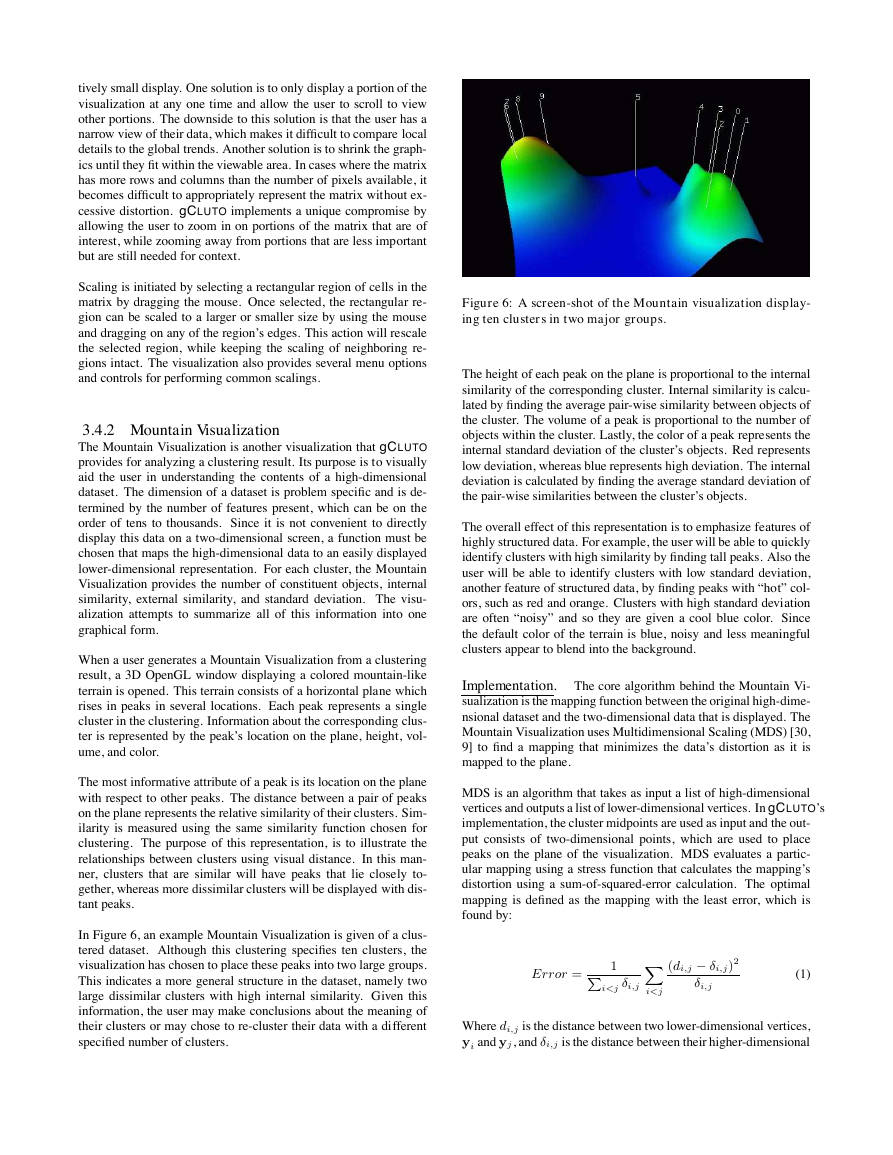
The Matrix visualization allows the user to interactively view, ex-
plore, and understand the clustering solution by zooming, querying,
and averaging arbitrary rows and columns. It represents the origi-
nal data matrix except with a few alterations. First, colors are used
to represent the values of the matrix. For example, dark red repre-
sents large positive values, while lighter shades are used for values
near zero. Conversely, shades of green are used for negative values.
Second, the rows of the matrix are reordered in order to display the
clusters found during clustering. Objects of the same cluster have
their rows placed consecutively and black horizontal lines separate
rows belonging to different clusters.
This display allows the user to visually inspect their data for pat-
terns. In an ideal clustering solution, rows belonging to the same
cluster should have relatively similar patterns of red and green. The
visualization emphasizes these patterns for the user by displaying
them in contiguous blocks. If the features represent a sequence, for
example measurements in a time-course experiment, then the user
can identify trends that occur across the features. The user may
Figure 4: Example solution report of a clustering of sports re-
lated documents. The sections of this report in order are clus-
tering options, cluster statistics, class distribution, and descrip-
tive and discriminating features.
�
Figure 5: A screen-shot of the Matrix visualization.
also be able to identify more questionable clusters by observing
stark dissimilarities between rows within a cluster.
In addition to the color matrix, the visualization also includes la-
bels and hierarchical trees located at the edges of the matrix. If the
user supplies labels with their data, then the rows of the matrix will
be labeled with object names and the columns with feature names.
If the user clusters their data with an agglomerative algorithm, then
the agglomerative tree will be displayed on the left-hand side of
the visualization. The user may also generate a hierarchical tree
even if a partitional clustering algorithm was used. In such cases,
gCLUTO performs additional agglomerative clustering within each
partitional cluster and a single agglomerative clustering of the clus-
ters themselves. Using the trees generated from these additional
clusterings, gCLUTO constructs a single hierarchical tree that con-
forms to the same cluster structure found with the partitional algo-
rithm. Lastly, the Matrix Visualization can also display a hierarchi-
cal tree called the feature tree, which is generated by performing
agglomerative clustering on the transpose of the data matrix.
Similar to visualizations in other clustering applications, the hier-
archical tree depicts relationships between objects by displaying
the order in which objects were merged in the agglomerative pro-
cess. Since merging is performed by descending pair-wise simi-
larity, objects that are near each other in the tree are more similar
than objects placed in distant locations. However, if users want
to draw conclusions about object similarities using the hierarchical
tree, they must keep in mind that a two-dimensional drawing of a
hierarchical tree is not unique. That is, for every parent node in
the tree, the two children nodes and their sub-trees can be drawn in
one of two possible orientations: top or bottom (note that gCLUTO
draws the hierarchical tree with children placed to the upper-right
or lower-right of their parents). gCLUTO removes this ambiguity
by explicitly ordering the visual position of each subtree by choos-
ing the set of orientations that maximizes the similarity between
objects placed in consecutive rows in the Matrix Visualization.
Manipulating the Matrix Visualization. Once the Matrix vi-
sualization is generated, users can further explore their results by
manipulating the visualization in several ways. First, the user may
collapse any set of rows or columns in the matrix by collapsing the
corresponding nodes in the hierarchical trees located above and to
the left of the matrix. By collapsing a node of the tree, the user can
hide all of the node’s descendants. In the matrix, the corresponding
rows that belong to the leaves of the collapsed sub-tree are replaced
by a single representative row. The representative row contains the
average vector of all of the hidden rows and, thus, summaries the
data in a condensed form. This feature is especially useful for large
datasets that are difficult to fully display on a computer monitor.
Columns can also be collapsed in a similar manner. When a rep-
resentative row crosses a representative column, the intersection is
a representative cell, which contains the average value of the cells
contained within the collapsed rectangular region.
A frequent use of row averaging is to view the cluster mid-point
vectors. This can be done either by collapsing the appropriate
nodes in the object hierarchical tree, or by selecting the “Show
Only Clusters” option from the “Matrix” menu. The user may also
quickly expand all collapsed nodes by choosing the “Show All Ob-
jects” option from the “Matrix” menu.
The last manipulation that is available to the user is scaling. A
common problem with viewing similar visualizations in other ap-
plications, is that it is difficult to represent a large dataset on a rela-
�
tively small display. One solution is to only display a portion of the
visualization at any one time and allow the user to scroll to view
other portions. The downside to this solution is that the user has a
narrow view of their data, which makes it difficult to compare local
details to the global trends. Another solution is to shrink the graph-
ics until they fit within the viewable area. In cases where the matrix
has more rows and columns than the number of pixels available, it
becomes difficult to appropriately represent the matrix without ex-
cessive distortion. gCLUTO implements a unique compromise by
allowing the user to zoom in on portions of the matrix that are of
interest, while zooming away from portions that are less important
but are still needed for context.
Scaling is initiated by selecting a rectangular region of cells in the
matrix by dragging the mouse. Once selected, the rectangular re-
gion can be scaled to a larger or smaller size by using the mouse
and dragging on any of the region’s edges. This action will rescale
the selected region, while keeping the scaling of neighboring re-
gions intact. The visualization also provides several menu options
and controls for performing common scalings.
3.4.2 Mountain Visualization
The Mountain Visualization is another visualization that gCLUTO
provides for analyzing a clustering result. Its purpose is to visually
aid the user in understanding the contents of a high-dimensional
dataset. The dimension of a dataset is problem specific and is de-
termined by the number of features present, which can be on the
order of tens to thousands. Since it is not convenient to directly
display this data on a two-dimensional screen, a function must be
chosen that maps the high-dimensional data to an easily displayed
lower-dimensional representation. For each cluster, the Mountain
Visualization provides the number of constituent objects, internal
similarity, external similarity, and standard deviation. The visu-
alization attempts to summarize all of this information into one
graphical form.
When a user generates a Mountain Visualization from a clustering
result, a 3D OpenGL window displaying a colored mountain-like
terrain is opened. This terrain consists of a horizontal plane which
rises in peaks in several locations. Each peak represents a single
cluster in the clustering. Information about the corresponding clus-
ter is represented by the peak’s location on the plane, height, vol-
ume, and color.
The most informative attribute of a peak is its location on the plane
with respect to other peaks. The distance between a pair of peaks
on the plane represents the relative similarity of their clusters. Sim-
ilarity is measured using the same similarity function chosen for
clustering. The purpose of this representation, is to illustrate the
relationships between clusters using visual distance. In this man-
ner, clusters that are similar will have peaks that lie closely to-
gether, whereas more dissimilar clusters will be displayed with dis-
tant peaks.
In Figure 6, an example Mountain Visualization is given of a clus-
tered dataset. Although this clustering specifies ten clusters, the
visualization has chosen to place these peaks into two large groups.
This indicates a more general structure in the dataset, namely two
large dissimilar clusters with high internal similarity. Given this
information, the user may make conclusions about the meaning of
their clusters or may chose to re-cluster their data with a different
specified number of clusters.
Figure 6: A screen-shot of the Mountain visualization display-
ing ten clusters in two major groups.
The height of each peak on the plane is proportional to the internal
similarity of the corresponding cluster. Internal similarity is calcu-
lated by finding the average pair-wise similarity between objects of
the cluster. The volume of a peak is proportional to the number of
objects within the cluster. Lastly, the color of a peak represents the
internal standard deviation of the cluster’s objects. Red represents
low deviation, whereas blue represents high deviation. The internal
deviation is calculated by finding the average standard deviation of
the pair-wise similarities between the cluster’s objects.
The overall effect of this representation is to emphasize features of
highly structured data. For example, the user will be able to quickly
identify clusters with high similarity by finding tall peaks. Also the
user will be able to identify clusters with low standard deviation,
another feature of structured data, by finding peaks with “hot” col-
ors, such as red and orange. Clusters with high standard deviation
are often “noisy” and so they are given a cool blue color. Since
the default color of the terrain is blue, noisy and less meaningful
clusters appear to blend into the background.
Implementation.
The core algorithm behind the Mountain Vi-
sualization is the mapping function between the original high-dime-
nsional dataset and the two-dimensional data that is displayed. The
Mountain Visualization uses Multidimensional Scaling (MDS) [30,
9] to find a mapping that minimizes the data’s distortion as it is
mapped to the plane.
MDS is an algorithm that takes as input a list of high-dimensional
vertices and outputs a list of lower-dimensional vertices. In gCLUTO’s
implementation, the cluster midpoints are used as input and the out-
put consists of two-dimensional points, which are used to place
peaks on the plane of the visualization. MDS evaluates a partic-
ular mapping using a stress function that calculates the mapping’s
distortion using a sum-of-squared-error calculation. The optimal
mapping is defined as the mapping with the least error, which is
found by:
X
1�
Error =
i


 2023年江西萍乡中考道德与法治真题及答案.doc
 2012年重庆南川中考生物真题及答案.doc
 2013年江西师范大学地理学综合及文艺理论基础考研真题.doc
 2020年四川甘孜小升初语文真题及答案I卷.doc
 2020年注册岩土工程师专业基础考试真题及答案.doc
 2023-2024学年福建省厦门市九年级上学期数学月考试题及答案.doc
 2021-2022学年辽宁省沈阳市大东区九年级上学期语文期末试题及答案.doc
 2022-2023学年北京东城区初三第一学期物理期末试卷及答案.doc
 2018上半年江西教师资格初中地理学科知识与教学能力真题及答案.doc
 2012年河北国家公务员申论考试真题及答案-省级.doc
 2020-2021学年江苏省扬州市江都区邵樊片九年级上学期数学第一次质量检测试题及答案.doc
 2022下半年黑龙江教师资格证中学综合素质真题及答案.doc