logo资料库

使用Julia语言编写计算程序.pdf

第1页 / 共99页
第2页 / 共99页
第3页 / 共99页
第4页 / 共99页
第5页 / 共99页
第6页 / 共99页
第7页 / 共99页
第8页 / 共99页
资料共99页,剩余部分请下载后查看
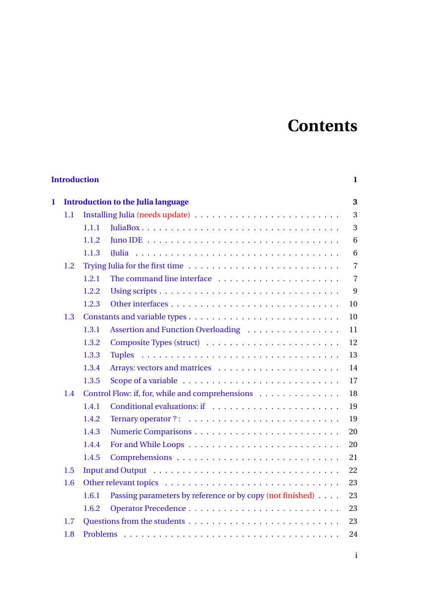
Contents
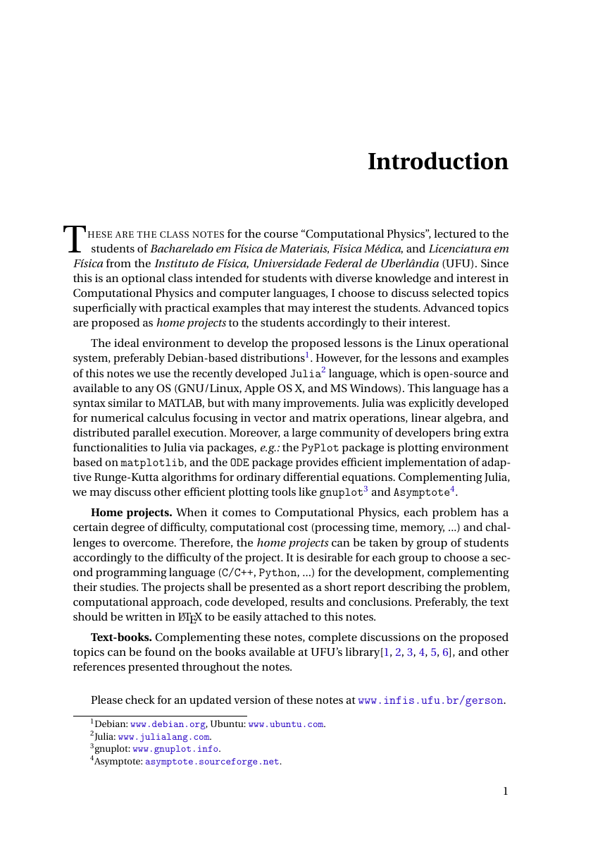
Introduction
Introduction to the Julia language
Installing Julia (needs update)
JuliaBox
Juno IDE
iJulia
Trying Julia for the first time
The command line interface
Essential commands, auto-complete, and command history
Using scripts
Other interfaces
Constants and variable types
Assertion and Function Overloading
Composite Types (struct)
Tuples
Arrays: vectors and matrices
Indexing an array or matrix
Concatenation
Scope of a variable
Control Flow: if, for, while and comprehensions
Conditional evaluations: if
Ternary operator ?:
Numeric Comparisons
For and While Loops
Comprehensions
Input and Output
Other relevant topics
Passing parameters by reference or by copy (not finished)
Operator Precedence
Questions from the students
Problems
Differential and Integral Calculus
Interpolation / Discretization
Numerical Integration - Quadratures
Polynomial Interpolations
Adaptive and multi-dimensional integration
Monte Carlo integration
Numerical Derivatives
Finite differences and Taylor series
Matrix Representation
Derivatives via convolution with a kernel
Other methods, Julia commands and packages for derivatives
Problems
Ordinary Differential Equations
Initial value problem: time-evolution
The Euler method
Runge-Kutta Methods
Stiff equations
Julia's ODE package
Boundary-value problems
Boundary conditions: Dirichlet and Neumann
The Sturm-Liouville problems
The Wronskian method
First step: find two linearly independent solutions of the homogeneous equation
Second step: find the particular solution of the inhomogeneous equation
Third step: impose the physical boundary conditions
Example: the Poisson equation via the Wronskian method
Schroedinger equations: transmission across a barrier
Non-linear differential equations
The shooting method
The eigenvalue problem
Oscillations on a string
Electron in a box
Method of finite differences
Problems
Fourier Series and Transforms
General properties of the Fourier transform
Numerical implementations
Discrete Fourier Transform (DFT)
Fast Fourier Transform (FFT)
Julia's native FFT
Applications of the FFT
Spectral analysis and frequency filters
Noise and frequency filters
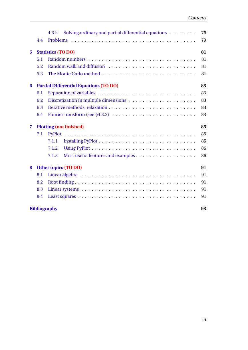
Solving ordinary and partial differential equations
Diffusion equation
Quantum operators in k-space, the split-step method
Problems
Statistics (TO DO)
Random numbers
Random walk and diffusion
The Monte Carlo method
Partial Differential Equations (TO DO)
Separation of variables
Discretization in multiple dimensions
Iterative methods, relaxation
Fourier transform (see §4.3.2)
Plotting (not finished)
PyPlot
Installing PyPlot
Using PyPlot
Most useful features and examples
Calling non-ported functions from Matplotlib
Latex
Subplot
Labels
Legends
Other plot elements
Saving into files (PNG, PDF, SVG, EPS, ...)
Animations
Other topics (TO DO)
Linear algebra
Root finding
Linear systems
Least squares
Bibliography
Gerson J. Ferreira Nanosciences Group www.infis.ufu.br/gnano Introduction to Computational Physics with examples in Julia DOI: 10.13140/RG.2.2.33138.30401 This is a draft! Please check for an updated version on http://www.infis.ufu.br/gerson Currently, I’m not working on this text. I’ll start to review and improve/finish some sections next semester. Institute of Physics, Federal University of Uberlândia October 5, 2016
Contents Introduction 1 Introduction to the Julia language 1.1 1.3.1 1.3.2 Composite Types (struct) 1.3.3 1.3.4 1.3.5 Installing Julia (needs update) . . . . . . . . . . . . . . . . . . . . . . . . . JuliaBox . . . . . . . . . . . . . . . . . . . . . . . . . . . . . . . . . . 1.1.1 1.1.2 Juno IDE . . . . . . . . . . . . . . . . . . . . . . . . . . . . . . . . . iJulia . . . . . . . . . . . . . . . . . . . . . . . . . . . . . . . . . . . 1.1.3 1.2 Trying Julia for the first time . . . . . . . . . . . . . . . . . . . . . . . . . . 1.2.1 The command line interface . . . . . . . . . . . . . . . . . . . . . 1.2.2 Using scripts . . . . . . . . . . . . . . . . . . . . . . . . . . . . . . . 1.2.3 Other interfaces . . . . . . . . . . . . . . . . . . . . . . . . . . . . . 1.3 Constants and variable types . . . . . . . . . . . . . . . . . . . . . . . . . . Assertion and Function Overloading . . . . . . . . . . . . . . . . . . . . . . . . . . . . . . . . . . . . . . . . . . . . . . . . . . . . . . . . . . . . . . . . . . . . . . . . . Tuples Arrays: vectors and matrices . . . . . . . . . . . . . . . . . . . . . Scope of a variable . . . . . . . . . . . . . . . . . . . . . . . . . . . 1.4 Control Flow: if, for, while and comprehensions . . . . . . . . . . . . . . 1.4.1 Conditional evaluations: if . . . . . . . . . . . . . . . . . . . . . . Ternary operator ?: . . . . . . . . . . . . . . . . . . . . . . . . . . 1.4.2 1.4.3 Numeric Comparisons . . . . . . . . . . . . . . . . . . . . . . . . . 1.4.4 For and While Loops . . . . . . . . . . . . . . . . . . . . . . . . . . 1.4.5 Comprehensions . . . . . . . . . . . . . . . . . . . . . . . . . . . . 1.5 . . . . . . . . . . . . . . . . . . . . . . . . . . . . . . . . Input and Output 1.6 Other relevant topics . . . . . . . . . . . . . . . . . . . . . . . . . . . . . . 1.6.1 Passing parameters by reference or by copy (not finished) . . . . 1.6.2 Operator Precedence . . . . . . . . . . . . . . . . . . . . . . . . . . 1.7 Questions from the students . . . . . . . . . . . . . . . . . . . . . . . . . . 1.8 Problems . . . . . . . . . . . . . . . . . . . . . . . . . . . . . . . . . . . . . 1 3 3 3 6 6 7 7 9 10 10 11 12 13 14 17 18 19 19 20 20 21 22 23 23 23 23 24 i
Introduction to Computational Physics Gerson J. Ferreira - INFIS - UFU - Brazil 2 Differential and Integral Calculus 2.1 Interpolation / Discretization . . . . . . . . . . . . . . . . . . . . . . . . . 2.2 Numerical Integration - Quadratures . . . . . . . . . . . . . . . . . . . . . Polynomial Interpolations . . . . . . . . . . . . . . . . . . . . . . . 2.2.1 2.2.2 Adaptive and multi-dimensional integration . . . . . . . . . . . . 2.2.3 Monte Carlo integration . . . . . . . . . . . . . . . . . . . . . . . . . . . . . . . . . . . . . . . . . . . . . . . . . . . . . 2.3.1 . . . . . . . . . . . . . . . . . 2.3.2 Matrix Representation . . . . . . . . . . . . . . . . . . . . . . . . . 2.3.3 Derivatives via convolution with a kernel . . . . . . . . . . . . . . 2.3.4 Other methods, Julia commands and packages for derivatives . 2.4 Problems . . . . . . . . . . . . . . . . . . . . . . . . . . . . . . . . . . . . . Finite differences and Taylor series 2.3 Numerical Derivatives 3 Ordinary Differential Equations 3.1 Initial value problem: time-evolution . . . . . . . . . . . . . . . . . . . . . 3.1.1 The Euler method . . . . . . . . . . . . . . . . . . . . . . . . . . . . 3.1.2 Runge-Kutta Methods . . . . . . . . . . . . . . . . . . . . . . . . . 3.1.3 Stiff equations . . . . . . . . . . . . . . . . . . . . . . . . . . . . . . Julia’s ODE package . . . . . . . . . . . . . . . . . . . . . . . . . . . 3.1.4 3.2 Boundary-value problems . . . . . . . . . . . . . . . . . . . . . . . . . . . 3.2.1 Boundary conditions: Dirichlet and Neumann . . . . . . . . . . . The Sturm-Liouville problems . . . . . . . . . . . . . . . . . . . . 3.2.2 The Wronskian method . . . . . . . . . . . . . . . . . . . . . . . . 3.2.3 3.2.4 Schroedinger equations: transmission across a barrier . . . . . . . . . . . . . . . . . . . . . . . . 3.2.5 Non-linear differential equations 3.3 The eigenvalue problem . . . . . . . . . . . . . . . . . . . . . . . . . . . . 3.3.1 Oscillations on a string . . . . . . . . . . . . . . . . . . . . . . . . . 3.3.2 Electron in a box . . . . . . . . . . . . . . . . . . . . . . . . . . . . 3.3.3 Method of finite differences . . . . . . . . . . . . . . . . . . . . . . 3.4 Problems . . . . . . . . . . . . . . . . . . . . . . . . . . . . . . . . . . . . . 4 Fourier Series and Transforms 4.1 General properties of the Fourier transform . . . . . . . . . . . . . . . . . 4.2 Numerical implementations . . . . . . . . . . . . . . . . . . . . . . . . . . 4.2.1 Discrete Fourier Transform (DFT) . . . . . . . . . . . . . . . . . . Fast Fourier Transform (FFT) . . . . . . . . . . . . . . . . . . . . . 4.2.2 4.2.3 Julia’s native FFT . . . . . . . . . . . . . . . . . . . . . . . . . . . . 4.3 Applications of the FFT . . . . . . . . . . . . . . . . . . . . . . . . . . . . . Spectral analysis and frequency filters . . . . . . . . . . . . . . . . 4.3.1 ii 27 27 30 31 33 34 35 35 37 38 39 39 43 44 46 47 49 52 53 53 55 57 59 61 62 63 63 64 65 69 71 72 72 72 73 75 75
Contents 4.3.2 Solving ordinary and partial differential equations . . . . . . . . 4.4 Problems . . . . . . . . . . . . . . . . . . . . . . . . . . . . . . . . . . . . . 5 Statistics (TO DO) 5.1 Random numbers . . . . . . . . . . . . . . . . . . . . . . . . . . . . . . . . 5.2 Random walk and diffusion . . . . . . . . . . . . . . . . . . . . . . . . . . 5.3 The Monte Carlo method . . . . . . . . . . . . . . . . . . . . . . . . . . . . 6 Partial Differential Equations (TO DO) Separation of variables . . . . . . . . . . . . . . . . . . . . . . . . . . . . . 6.1 6.2 Discretization in multiple dimensions . . . . . . . . . . . . . . . . . . . . 6.3 Iterative methods, relaxation . . . . . . . . . . . . . . . . . . . . . . . . . . 6.4 Fourier transform (see §4.3.2) . . . . . . . . . . . . . . . . . . . . . . . . . 7 Plotting (not finished) 7.1 PyPlot . . . . . . . . . . . . . . . . . . . . . . . . . . . . . . . . . . . . . . . 7.1.1 Installing PyPlot . . . . . . . . . . . . . . . . . . . . . . . . . . . . . 7.1.2 Using PyPlot . . . . . . . . . . . . . . . . . . . . . . . . . . . . . . . 7.1.3 Most useful features and examples . . . . . . . . . . . . . . . . . . 8 Other topics (TO DO) 8.1 Linear algebra . . . . . . . . . . . . . . . . . . . . . . . . . . . . . . . . . . 8.2 Root finding . . . . . . . . . . . . . . . . . . . . . . . . . . . . . . . . . . . . 8.3 Linear systems . . . . . . . . . . . . . . . . . . . . . . . . . . . . . . . . . . 8.4 Least squares . . . . . . . . . . . . . . . . . . . . . . . . . . . . . . . . . . . Bibliography 76 79 81 81 81 81 83 83 83 83 83 85 85 85 86 86 91 91 91 91 91 93 iii
Introduction THESE ARE THE CLASS NOTES for the course “Computational Physics”, lectured to the students of Bacharelado em Física de Materiais, Física Médica, and Licenciatura em Física from the Instituto de Física, Universidade Federal de Uberlândia (UFU). Since this is an optional class intended for students with diverse knowledge and interest in Computational Physics and computer languages, I choose to discuss selected topics superficially with practical examples that may interest the students. Advanced topics are proposed as home projects to the students accordingly to their interest. The ideal environment to develop the proposed lessons is the Linux operational system, preferably Debian-based distributions1. However, for the lessons and examples of this notes we use the recently developed Julia2 language, which is open-source and available to any OS (GNU/Linux, Apple OS X, and MS Windows). This language has a syntax similar to MATLAB, but with many improvements. Julia was explicitly developed for numerical calculus focusing in vector and matrix operations, linear algebra, and distributed parallel execution. Moreover, a large community of developers bring extra functionalities to Julia via packages, e.g.: the PyPlot package is plotting environment based on matplotlib, and the ODE package provides efficient implementation of adap- tive Runge-Kutta algorithms for ordinary differential equations. Complementing Julia, we may discuss other efficient plotting tools like gnuplot3 and Asymptote4. Home projects. When it comes to Computational Physics, each problem has a certain degree of difficulty, computational cost (processing time, memory, ...) and chal- lenges to overcome. Therefore, the home projects can be taken by group of students accordingly to the difficulty of the project. It is desirable for each group to choose a sec- ond programming language (C/C++, Python, ...) for the development, complementing their studies. The projects shall be presented as a short report describing the problem, computational approach, code developed, results and conclusions. Preferably, the text should be written in LATEX to be easily attached to this notes. Text-books. Complementing these notes, complete discussions on the proposed topics can be found on the books available at UFU’s library[1, 2, 3, 4, 5, 6], and other references presented throughout the notes. Please check for an updated version of these notes at www.infis.ufu.br/gerson. 1Debian: www.debian.org, Ubuntu: www.ubuntu.com. 2Julia: www.julialang.com. 3gnuplot: www.gnuplot.info. 4Asymptote: asymptote.sourceforge.net. 1
分享到:
收藏