光线追踪入门技术.pdf-资料库

zzh5756712-10658463-4744302543365800458.pdf-第1页.png

第1页 / 共50页

zzh5756712-10658463-4744302543365800458.pdf-第2页.png

第2页 / 共50页

zzh5756712-10658463-4744302543365800458.pdf-第3页.png

第3页 / 共50页

zzh5756712-10658463-4744302543365800458.pdf-第4页.png

第4页 / 共50页

zzh5756712-10658463-4744302543365800458.pdf-第5页.png

第5页 / 共50页

zzh5756712-10658463-4744302543365800458.pdf-第6页.png

第6页 / 共50页

zzh5756712-10658463-4744302543365800458.pdf-第7页.png

第7页 / 共50页

zzh5756712-10658463-4744302543365800458.pdf-第8页.png

第8页 / 共50页

Ray Tracing: The Next Week Peter Shirley Version 1.42 Copyright 2018. Peter Shirley. All rights reserved. Chapter 0: Overview In Ray Tracing In One Weekend, you built a simple brute force path tracer. In this installment we’ll add textures, volumes (like fog), rectangles, instances, lights, and support for lots of objects using a BVH. When done, you’ll have a “real” ray tracer. A heuristic in ray tracing that many people-- including me-- believe, is that most optimizations complicate the code without delivering much speedup. What I will do in this mini-book is go with the simplest approach in each design decision I make. Check www.in1weekend.com for readings and references to a more sophisticated approach. However, I strongly encourage you to do no premature optimization; if it doesn’t show up high in the execution time profile, it doesn’t need optimization until all the features are supported! The two hardest parts of this book are the BVH and the Perlin textures. This is why the title suggests you take a week rather than a weekend for this endeavor. But you can save those for last if you want a weekend project. Order is not very important for the concepts presented in this book, and without BVH and Perlin texture you will still get a Cornell Box! Acknowledgments: Thanks to Becker for his many helpful comments on the draft and to Matthew Heimlich for spotting a critical motion blur error. Thanks to Andrew Kensler, Thiago Ize, and Ingo Wald for advice on ray-AABB tests. Thanks to David Hart and Grue Debry for help with a bunch of the details. Thanks to Jean Buckley for editing. Chapter 1: Motion Blur When you decided to ray trace, you decided visual quality was worth more run-time. In your fuzzy reflection and defocus blur you needed multiple samples per pixel. Once you have taken a

step down that road, the good news is that almost all effects can be brute-forced. Motion blur is certainly one of those. In a real camera, the shutter opens and stays open for a time interval, and the camera and objects may move during that time. Its really an average of what the camera sees over that interval that we want. We can get a random estimate by sending each ray at some random time when the shutter is open. As long as the objects are where they should be at that time, we can get the right average answer with a ray that is at exactly a single time. This is fundamentally why random ray tracing tends to be simple. The basic idea is to generate rays at random times while the shutter is open and intersect the model at that one time. The way it is usually done is to have the camera move and the objects move, but have each ray exist at exactly one time. This way the “engine” of the ray tracer can just make sure the objects are where they need to be for the ray, and the intersection guts don’t change much. 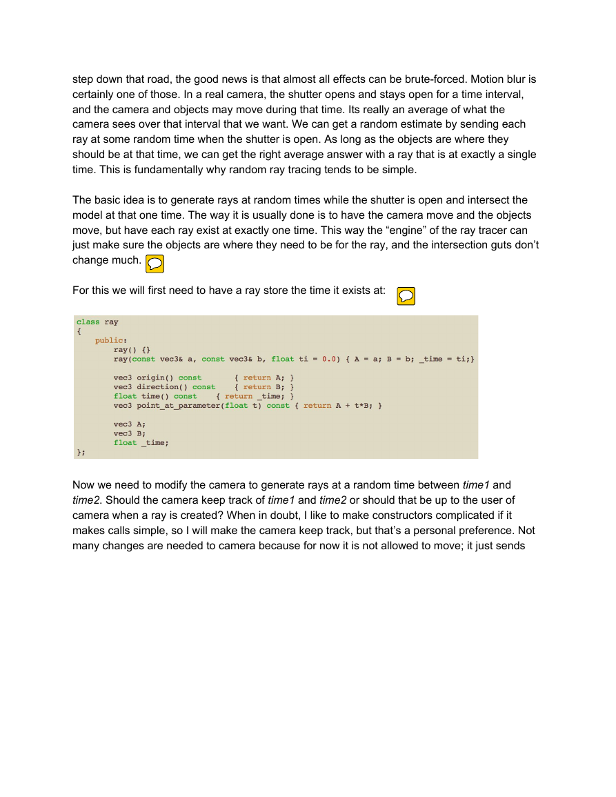For this we will first need to have a ray store the time it exists at: Now we need to modify the camera to generate rays at a random time between time1 and time2. Should the camera keep track of time1 and time2 or should that be up to the user of camera when a ray is created? When in doubt, I like to make constructors complicated if it makes calls simple, so I will make the camera keep track, but that’s a personal preference. Not many changes are needed to camera because for now it is not allowed to move; it just sends

out rays over a time period. We also need a moving object. I’ll create a sphere class that has its center move linearly from center0 at time0 to center1 at time1. Outside that time interval it continues on, so those times need not match up with the camera aperture open close. An alternative to making a new moving sphere class is to just make them all move and have the stationary ones have the same begin and end point. I’m on the fence about that trade-off between fewer classes and more efficient stationary spheres, so let your design taste guide you.

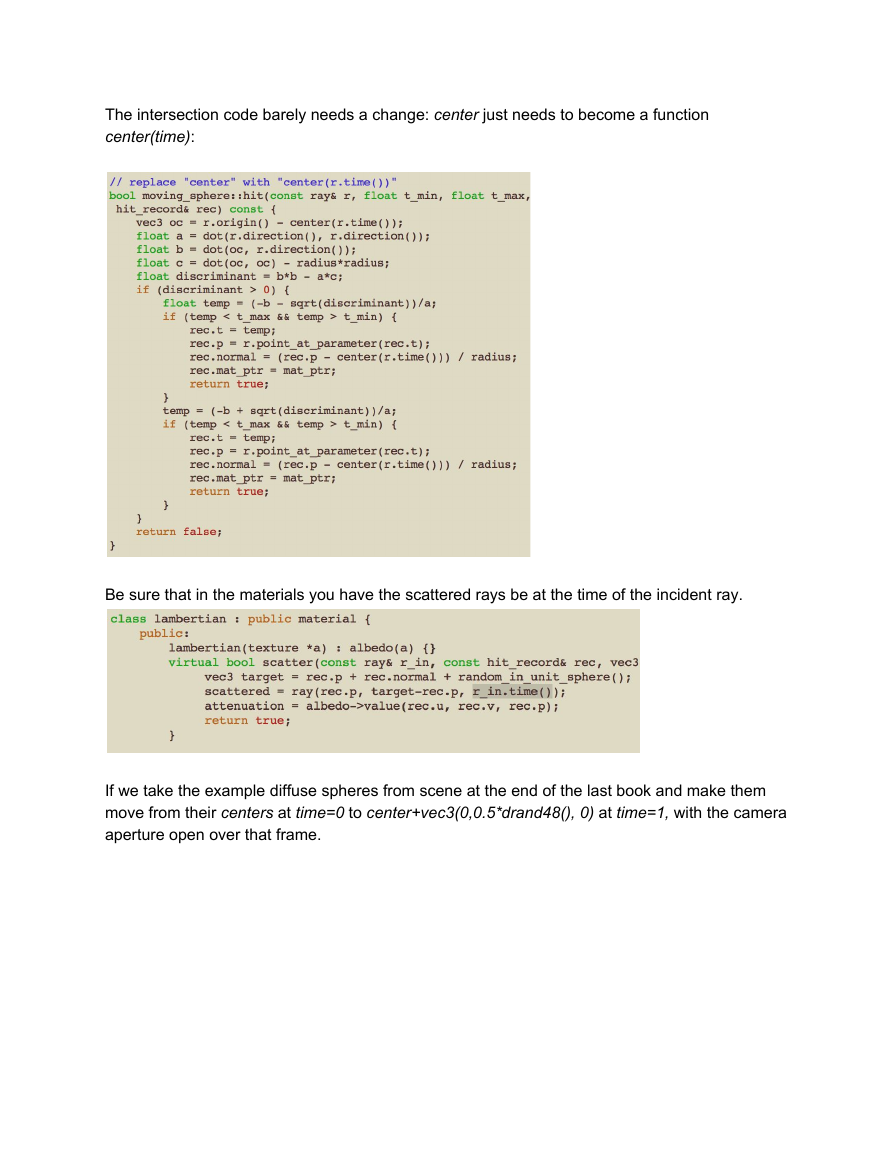
The intersection code barely needs a change: center just needs to become a function center(time): Be sure that in the materials you have the scattered rays be at the time of the incident ray. If we take the example diffuse spheres from scene at the end of the last book and make them move from their centers at time=0 to center+vec3(0,0.5*drand48(), 0) at time=1, with the camera aperture open over that frame.

And with these viewing parameters gives:

Chapter 2: Bounding Volume Hierarchies This part is by far the most difficult and involved part of the ray tracer we are working on. I am sticking it in Chapter 2 so the code can run faster, and because it refactors hitable a little, and when I add rectangles and boxes we won't have to go back and refactor them. The ray-object intersection is the main time-bottleneck in a ray tracer, and the time is linear with the number of objects. But it’s a repeated search on the same model, so we ought to be able to make it a logarithmic search in the spirit of binary search. Because we are sending millions to billions of rays on the same model, we can do an analog of sorting the model and then each ray intersection can be a sublinear search. The two most common families of sorting are to 1) divide the space, and 2) divide the objects. The latter is usually much easier to code up and just as fast to run for most models. The key idea of a bounding volume over a set of primitives is to find a volume that fully encloses (bounds) all the objects. For example, suppose you computed a bounding sphere of 10 objects. Any ray that misses the bounding sphere definitely misses all ten objects. If the ray hits the bounding sphere, then it might hit one of the ten objects. So the bounding code is always of the form: if (ray hits bounding object) return whether ray hits bounded objects else return false A key thing is we are dividing objects into subsets. We are not dividing the screen or the volume. Any object is in just one bounding volume, but bounding volumes can overlap. To make things sub-linear we need to make the bounding volumes hierarchical. For example, if we divided a set of objects into two groups, red and blue, and used rectangular bounding volumes, we’d have:

Note that the blue and red bounding volumes are contained in the purple one, but they might overlap, and they are not ordered-- they are just both inside. So the tree shown on the right has no concept of ordering in the left and right children; they are simply inside. The code would be: if (hits purple) hit0 = hits blue enclosed objects hit1 = hits red enclosed objects if (hit0 or hit1) return true and info of closer hit return false To get that all to work we need a way to make good divisions, rather than bad ones, and a way to intersect a ray with a bounding volume. A ray bounding volume intersection needs to be fast, and bounding volumes need to be pretty compact. In practice for most models, axis-aligned boxes work better than the alternatives, but this design choice is always something to keep in mind if you encounter unusual types of models. From now on we will call axis-aligned bounding rectangular parallelepiped (really, that is what they need to be called if precise) axis-aligned bounding boxes, or AABBs. Any method you want to use to intersect a ray with an AABB is fine. And all we need to know is whether or not we hit it; we don’t need hit points or normals or any of that stuff that we need for an object we want to display. 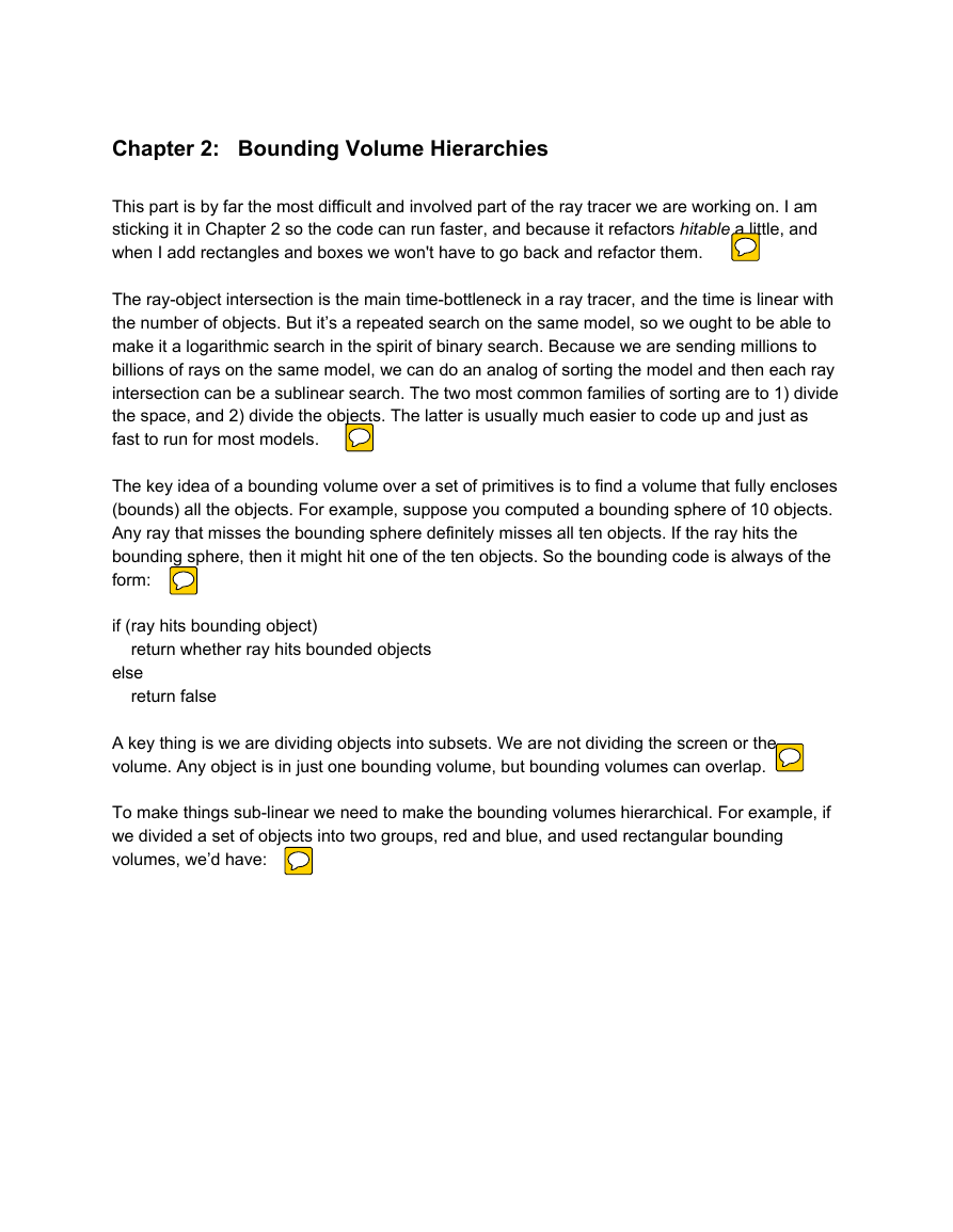Most people use the “slab” method. This is based on the observation that an n-dimensional AABB is just the intersection of n axis-aligned intervals, often called “slabs’’. An interval is just the points between two endpoints, e.g., x such that 3 < x < 5, or more succinctly x in (3,5). In 2D, two intervals overlapping makes a 2D AABB (a rectangle):

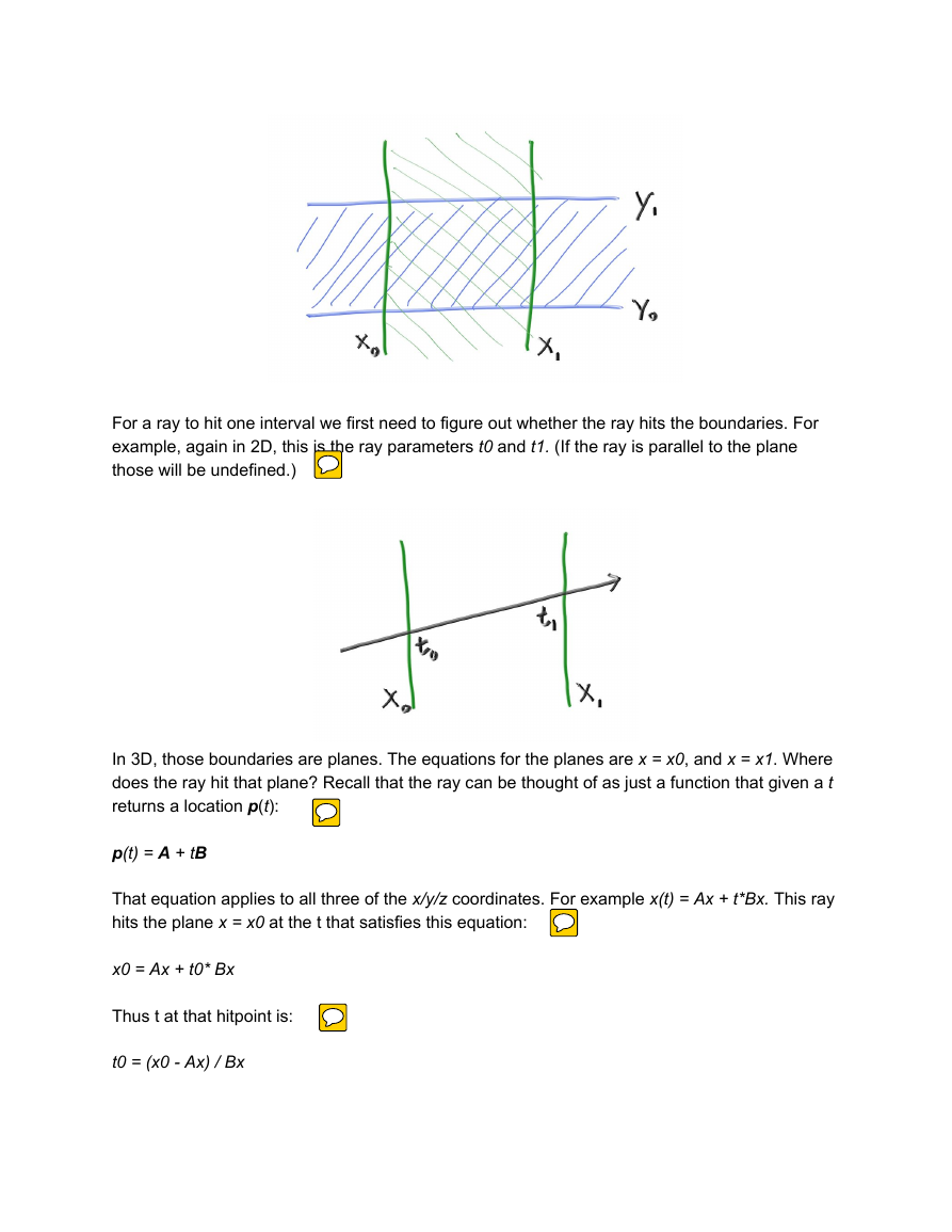
For a ray to hit one interval we first need to figure out whether the ray hits the boundaries. For example, again in 2D, this is the ray parameters t0 and t1. (If the ray is parallel to the plane those will be undefined.) In 3D, those boundaries are planes. The equations for the planes are x = x0, and x = x1. Where does the ray hit that plane? Recall that the ray can be thought of as just a function that given a t returns a location p(t): p(t) = A + tB That equation applies to all three of the x/y/z coordinates. For example x(t) = Ax + t*Bx. This ray hits the plane x = x0 at the t that satisfies this equation: x0 = Ax + t0* Bx Thus t at that hitpoint is: t0 = (x0 - Ax) / Bx

资料库

光线追踪入门技术.pdf

相关推荐

开发技术

热门标签

最新资料