Available online at www.sciencedirect.com
Automatica 40 (2004) 1017 – 1023
www.elsevier.com/locate/automatica
Multi-sensor optimal information fusion Kalman !lter�
Brief paper
Shu-Li Sun∗, Zi-Li Deng
Department of Automation, Heilongjiang University, P.O. Box 229, Harbin 150080, People’s Republic of China
Received 4 November 2002; received in revised form 27 December 2003; accepted 16 January 2004
Abstract
This paper presents a new multi-sensor optimal information fusion criterion weighted by matrices in the linear minimum variance
sense, it is equivalent to the maximum likelihood fusion criterion under the assumption of normal distribution. Based on this optimal
fusion criterion, a general multi-sensor optimal information fusion decentralized Kalman !lter with a two-layer fusion structure is given
for discrete time linear stochastic control systems with multiple sensors and correlated noises. The !rst fusion layer has a netted parallel
structure to determine the cross covariance between every pair of faultless sensors at each time step. The second fusion layer is the fusion
center that determines the optimal fusion matrix weights and obtains the optimal fusion !lter. Comparing it with the centralized !lter,
the result shows that the computational burden is reduced, and the precision of the fusion !lter is lower than that of the centralized !lter
when all sensors are faultless, but the fusion !lter has fault tolerance and robustness properties when some sensors are faulty. Further, the
precision of the fusion !lter is higher than that of each local !lter. Applying it to a radar tracking system with three sensors demonstrates
its e8ectiveness.
? 2004 Elsevier Ltd. All rights reserved.
Keywords: Multisensor; Information fusion; Linear minimum variance; Maximum likelihood; Optimal information fusion Kalman !lter; Fault tolerance;
Radar tracking system
1. Introduction
The information fusion Kalman !ltering theory has been
studied and widely applied to integrated navigation systems
for maneuvering targets, such as airplanes, ships, cars and
robots. When multiple sensors measure the states of the same
stochastic system, generally we have two di8erent types
of methods to process the measured sensor data. The !rst
method is the centralized !lter (Willner, Chang, & Dunn,
1976) where all measured sensor data are communicated to
a central site for processing. The advantage of this method
is that it involves minimal information loss. However, it can
result in severe computational overhead due to overloading
of the !lter with more data than it can handle. Consequently,
the overall centralized !lter may be unreliable or su8er from
poor accuracy and stability when there is severe data fault.
� This paper was not presented at any IFAC meeting. This paper was
recommended for publication in revised form by Associate Editor Marco
Campi under the direction of Editor Tamer Ba@sar.
∗ Corresponding author. Tel.: +86-0451-86622910.
E-mail address: sunsl@hlju.edu.cn (S.-L. Sun).
0005-1098/$ - see front matter ? 2004 Elsevier Ltd. All rights reserved.
doi:10.1016/j.automatica.2004.01.014
The second method is the decentralized !lter where the in-
formation from local estimators can yield the global optimal
or suboptimal state estimate according to certain informa-
tion fusion criterion. The advantage of this method is that
the requirements of communication and memory space at
the fusion center are broadened, and the parallel structures
would lead to increase in the input data rates. Furthermore,
decentralization leads to easy fault detection and isolation.
However, the precision of the decentralized !lter is gener-
ally lower than that of the centralized !lter when there is
no data fault. Various decentralized and parallel versions of
the Kalman !lter and their applications have been reported
(Kerr, 1987; Hashmipour, Roy, & Laub, 1988), including
the federated square-root !lter of Carlson (1990). But to
some extent, his !lter has conservatism because of using
the upper bound of the process noise variance matrix in-
stead of process noise variance matrix itself, and assuming
the initial estimation errors to be uncorrelated. Roy and Iltis
(1991) give a decentralized static !lter for the linear system
with correlated measurement noises. Kim (1994) gives an
optimal fusion !lter under the assumption of normal distri-
bution based on the maximum likelihood sense for systems
�
1018
S.-L. Sun, Z.-L. Deng / Automatica 40 (2004) 1017 – 1023
with multiple sensors, and assumes the process noise to be
independent of measurement noises. Saha (1996,1998) dis-
cusses the steady-state fusing problem. Deng and Qi (2000)
give a multi-sensor fusion criterion weighted by scalars. But
the assumption for the estimation errors among the local
subsystems to be uncorrelated does not accord with the gen-
eral case. Qiang and Harris (2001) discuss the functional
equivalence of two measurement fusion methods, where the
second method requires the measurement matrices to be of
identical size.
In this paper, the result of the maximum likelihood fu-
sion criterion under the normal density function, which is
presented by Kim (1994), is re-derived as an optimal in-
formation fusion criterion weighted by matrices in the lin-
ear minimum variance sense. Based on the fusion crite-
rion, an optimal information fusion decentralized !lter with
fault tolerance and robustness properties is given for discrete
time-varying linear stochastic control systems with multi-
ple sensors and correlated noises. It has a two-layer fusion
structure. The !rst fusion layer has a netted parallel struc-
ture to determine the cross covariance between every pair of
faultless sensors at each time step. The second fusion layer
is the fusion center that fuses the estimates and variances
of all local subsystems, and the cross covariance among the
local subsystems from the !rst fusion layer to determine the
optimal matrix weights and yield the optimal fusion !lter.
2. Problem formulation
Consider the discrete time-varying linear stochastic con-
trol system with l sensors
x(t + 1) = (t)x(t) + B(t)u(t) + (t)w(t);
(1)
i = 1; 2; : : : ; l;
yi(t) = Hi(t)x(t) + vi(t);
(2)
where x(t)∈ Rn is the state, yi(t)∈ Rmi is the measurement,
u(t)∈ Rp is a known control input, w(t)∈ Rr, vi(t)∈ Rmi
are white noises, and (t); B(t); (t); Hi(t) are time-varying
matrices with compatible dimensions.
In the following, In denotes the n× n identity matrix, and
0 denotes the zero matrix with compatible dimension.
Assumption 1. w(t) and vi(t), i = 1; 2; : : : ; l are correlated
white noises with zero mean and
tk;
(3)
E
w(t)
vi(t)
[ wT(k)
vT
i (k) ]
=
Si(t)
Q(t)
ST
i (t) Ri(t)
E[vi(t)vT
j (k)] = Sij(t)tk;
i = j;
Assumption 2. The initial state x(0) is independent of w(t)
and vi(t), i = 1; 2; : : : ; l, and
Ex(0) = 0;
E[(x(0) − 0)(x(0) − 0)T] = P0:
(4)
Our aim is to !nd the optimal (i.e. linear minimum vari-
ance) information fusion Kalman !lter ˆxo(t|t) of the state
x(t) based on measurements (yi(t); : : : ; yi(1)), i =1; 2; : : : ; l,
which will satisfy the following performances:
(a) Unbiasedness, namely, E ˆxo(t|t) = Ex(t).
(b) Optimality, namely, to !nd the optimal matrix weights
OAi(t), i = 1; 2; : : : ; l, to minimize the trace of the fusion
!ltering error variance, i.e. tr[Po(t|t)]=min{tr[P(t|t)]},
where the symbol tr denotes the trace of a matrix, Po(t|t)
denotes the variance of the optimal fusion !lter with
matrix weights and P(t|t) denotes the variance of an
arbitrary fusion !lter with matrix weights.
3. Optimal information fusion criterion in the linear
minimum variance sense
In 1994, Kim provides a maximum likelihood fusion cri-
terion under the assumption of standard normal distribution.
Here we will derive the same result in the linear minimum
variance sense, where the restrictive assumption of normal
distribution is avoided. For simplicity, time t is dropped in
the following derivation.
Theorem 1. Let ˆxi, i = 1; 2; : : : ; l be unbiased estimators
of an n-dimensional stochastic vector x. Let the estimation
errors be ˜xi=x− ˆxi, i=1; 2; : : : ; l. Assume that ˜xi and ˜xj, (i =
j) are correlated, and the variance and cross covariance
matrices are denoted by Pii (i.e. Pi) and Pij, respectively.
Then the optimal fusion (i.e. linear minimum variance)
estimator with matrix weights is given as
ˆxo = OA1 ˆx1 + OA2 ˆx2 + ··· + OAl ˆxl;
where the optimal matrix weights OAi, i=1; 2; : : : ; l are com-
puted by
OA = −1e(eT−1e)−1;
(6)
where =(Pij), i; j=1; 2; : : : ; l is an nl×nl symmetric posi-
tive de9nite matrix, OA=[ OA1; OA2; : : : ; OAl]T and e=[In; : : : ; In]T
are both nl × n matrices. The corresponding variance of
the optimal information fusion estimator is computed by
Po = (eT−1e)−1
and we have the conclusion Po 6 Pi, i = 1; 2; : : : ; l.
(5)
(7)
where the symbol E denotes the mathematical expecta-
tion, the superscript T denotes the transpose, and tk is the
Kronecker delta function.
Proof. Introducing the synthetically unbiased estimator
ˆx = A1 ˆx1 + A2 ˆx2 + ··· + Al ˆxl;
(8)
�
S.-L. Sun, Z.-L. Deng / Automatica 40 (2004) 1017 – 1023
1019
where Ai; i = 1; 2; : : : ; l are arbitrary matrices. From the un-
biasedness assumption, we have E ˆx = Ex, E ˆxi = Ex, i =
1; 2; : : : ; l. Taking the expectation of both sides of (8) yields
A1 + A2 + ··· + Al = In:
(9)
l
l
From (8) and (9) we have the fusion estimation error ˜x=x−
i=1 Ai(x − ˆxi) =
i=1 Ai ˜xi. Let A = [A1; A2; : : : ; Al]T,
ˆx =
so the error variance matrix of the fusion estimator is
where ei = [0; : : : ; In; : : : ; 0]T is an nl × n matrix whose ith
block place is an In and others are n×n block zero matrices.
The condition of the equality to hold in (16) is that Pi = Pji,
j = 1; 2; : : : ; l.
This proof is completed.
4. Optimal information fusion decentralized Kalman
lter with a two-layer fusion structure
P = E( ˜x ˜xT) = ATA
and the performance index J = tr(P) becomes
J = tr(ATA):
(10)
(11)
Under Assumptions 1 and 2, the ith local sensor subsys-
tem of system (1)–(2) with multiple sensors has the local
optimal Kalman !lter (Anderson & Moore, 1979)
ˆxi(t + 1|t + 1) = ˆxi(t + 1|t) + Ki(t + 1)&i(t + 1);
(17)
The problem is to !nd the optimal fusion matrix weights
OAi, i = 1; 2; : : : ; l under restriction (9) to minimize the per-
formance index (11). Applying the Lagrange multiplier
method, we introduce the auxiliary function
F = J + 2 tr[!(ATe − In)];
(12)
where ! = ("ij) is an n × n matrix. Set @F=@A|A= OA = 0, and
note that T = , we have
OA + e! = 0:
(13)
Combining (13) with (9) yields the matrix equation as
=
;
(14)
eT
e
0
OA
!
0
In
where ; e; OA are de!ned above. is a symmetric positive
de!nite matrix, hence eT−1e is nonsingular. Using the for-
mula of the inverse matrix (Xu, 2001), we have
−1
OA
!
=
=
e
0
0
eT
In
−1e(eT−1e)−1
−(eT−1e)−1
(15)
which yields (6). Substituting (6) into (10) yields the op-
timal information fusion estimation error variance matrix
as (7). The following is the derivation of Po 6 Pi. In fact,
applying Schwartz matrix inequality, we have
Po = (eT−1e)−1 = [(−1=2e)T(1=2ei)]T
×[(−1=2e)T(−1=2e)]−1[(−1=2e)T(1=2ei)]
6 (1=2ei)T(1=2ei) = Pi;
(16)
ˆxi(t + 1|t) = Oi(t) ˆxi(t|t) + B(t)u(t) + Ji(t)yi(t);
&i(t + 1) = yi(t + 1) − Hi(t + 1) ˆxi(t + 1|t);
Ki(t + 1) = Pi(t + 1|t)H T
×Pi(t + 1|t)H T
i (t + 1)[Hi(t + 1)
i (t + 1) + Ri(t + 1)]−1;
Pi(t + 1|t) = Oi(t)Pi(t|t) OT
×[Q(t) − Si(t)R−1
i
i (t) + (t)
(t)ST
i (t)]T(t);
(18)
(19)
(20)
(21)
Pi(t + 1|t + 1) = [In − Ki(t + 1)Hi(t + 1)]Pi(t + 1|t);
(22)
Pi(0|0) = P0;
ˆxi(0|0) = 0;
where Oi(t) = (t) − Ji(t)Hi(t), Ji(t) = (t)Si(t)R−1
(t).
Pi(t|t) and Pi(t+1|t) are the !ltering and !rst-step prediction
error variance matrices, respectively, Ki(t) is the !ltering
gain matrix, and &i(t) is the innovation process, for the ith
sensor subsystem, i = 1; 2; : : : ; l.
(23)
i
Since !ltering errors of the ith and the jth subsystems are
correlated, we have the following Theorem 2.
Theorem 2. Under Assumptions 1 and 2, the local Kalman
9ltering error cross covariance between the ith and the jth
sensor subsystems has the following recursive form:
Pij(t + 1|t + 1) = [In − Ki(t + 1)Hi(t + 1)]
j (t)
×{ Oi(t)Pij(t|t) OT
+(t)Q(t)T(t) − Jj(t)Rj(t)J T
−Ji(t)Ri(t)J T
i (t) + Ji(t)Sij(t)J T
+ Oi(t)Ki(t)[Sij(t)J T
j (t)
j (t)
j (t)
�
1020
S.-L. Sun, Z.-L. Deng / Automatica 40 (2004) 1017 – 1023
i (t)T(t)] + [Ji(t)Sij(t)
−ST
−(t)Sj(t)]K T
×[In − Kj(t + 1)Hj(t + 1)]T
+Ki(t + 1)Sij(t + 1)K T
j (t) OT
j (t)}
(24)
where Pij(t|t), i; j = 1; 2; : : : ; l (i = j) are the 9ltering error
cross covariance matrices between the ith and jth sensor
subsystems, and the initial values Pij(0|0) = P0.
j (t + 1);
Proof. For the ith sensor subsystem, we have the !ltering
error equation as follows (Anderson & Moore, 1979):
˜xi(t + 1|t + 1) = [In − Ki(t + 1)Hi(t + 1)][ Oi(t) ˜xi(t|t)
+ Owi(t)] − Ki(t + 1)vi(t + 1);
(25)
where Owi(t) = (t)w(t) − Ji(t)vi(t), ˜xi(t|t) = x(t) − ˆxi(t|t),
i=1; 2; : : : ; l. Since the !ltering error ˜xi(t|t) consists of linear
combination of (w(t−1); : : : ; w(0); x(0); vi(t); : : : ; vi(1)), ap-
plying the projection property (Anderson & Moore, 1979),
we have ˜xi(t|t) ⊥ vj(t +1), i; j =1; 2; : : : ; l, where ⊥ denotes
orthogonality. Using Assumption 1 and (25) yields the !l-
tering error cross covariance matrix between the ith and the
jth sensor subsystems as follows:
Pij(t + 1|t + 1) = [In − Ki(t + 1)Hi(t + 1)]
×{ Oi(t)Pij(t|t) OT
+E[ Owi(t) OwT
j (t)
j (t)] + Oi(t)E[ ˜xi(t|t) OwT
j (t|t)] OT
j (t)}
j (t)]
+E[ Owi(t) ˜xT
×[In − Kj(t + 1)Hj(t + 1)]T
+Ki(t + 1)Sij(t + 1)K T
j (t + 1);
(26)
where
E[ Owi(t) OwT
j (t)] = (t)Q(t)T(t) − (t)Sj(t)J T
j (t)
i (t)T(t) + Ji(t)Sij(t)J T
−Ji(t)ST
j (t); (27)
E[ ˜xi(t|t) OwT
j (t)] = E{[(In − Ki(t)Hi(t))
× ˜xi(t|t − 1) − Ki(t)vi(t)]
×[(t)w(t) − Jj(t)vj(t)]T}
j (t) − Ki(t)ST
= Ki(t)Sij(t)J T
i (t)T(t): (28)
In (28), ˜xi(t|t − 1) ⊥ w(t) and ˜xi(t|t − 1) ⊥ vj(t) are used.
In a similar manner, we have
j (t|t)] = Ji(t)Sij(t)K T
j (t) − (t)Sj(t)K T
E[ Owi(t) ˜xT
j (t):
(29)
Substituting (27)–(29) into (26) yields (24). Using (4) and
(23) yields the initial value Pij(0|0) = P0.
Corollary 1 (Bar-Shalom, 1981). In Theorem 2, if Si(t)=0,
Sij(t) = 0, the cross covariance Pij(t + 1|t + 1) is simply
given by
Pij(t + 1|t + 1) = [In − Ki(t + 1)Hi(t + 1)]
×[(t)Pij(t|t)T(t) + (t)Q(t)T(t)]
×[In − Kj(t + 1)Hj(t + 1)]T:
(30)
Proof. This follows directly from Theorem 2.
Based on Theorems 1 and 2, we easily obtain the follow-
ing corollary.
Corollary 2. For system (1)–(2) under Assumptions 1 and
2, we have the optimal information fusion decentralized
Kalman 9lter as
ˆxo(t|t) = OA1(t) ˆx1(t|t) + OA2(t)
× ˆx2(t|t) + ··· + OAl(t) ˆxl(t|t);
(31)
where ˆxi(t|t), i =1; 2; : : : ; l, are computed by (17)–(23), the
optimal matrix weights OAi(t), i=1; 2; : : : ; l are computed by
(6) and the optimal fusion variance Po(t|t) is computed by
(7). The 9ltering error variance Pi(t|t) and cross covariance
Pij(t|t), (i = j) of the local subsystems are computed by
(22) and (24), respectively.
Proof. This follows directly from Theorems 1 and 2.
The optimal information fusion decentralized !lter (31)
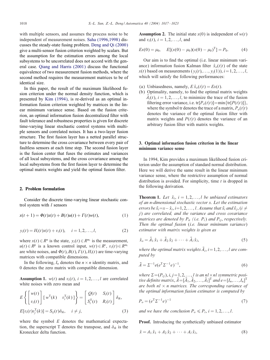
has a two-layer fusion structure as shown in Fig. 1.
In Fig. 1, every sensor subsystem independently estimates
the states, respectively and makes fault detection. The clas-
sical approaches for fault detection have WSSR (Willsky,
1976) and U veri!cation (Mehra & Peschon, 1971). If any
sensor subsystem is faulty by detection, it is isolated and
restored. Otherwise, it is sent to the !rst fusion layer with
a netted parallel structure in which the estimation errors of
every pair of sensors are fused to determine the cross co-
variance between them at each time step, at the same time
the estimates and variances are sent to the second fusion
layer. The second fusion layer is the !nal fusion center in
which the estimates and variance matrices of all faultless
local subsystems, and the cross covariance matrices among
the faultless local subsystems from the !rst fusion layer are
fused by Theorem 1 to determine the optimal matrix weights
and obtain the optimal fusion !lter. On the other hand, af-
ter the faulty sensors are restored, they can be re-joined the
parallel fusion structure. Since the decentralized structure is
used, the computational burden in the fusion center is re-
duced, and the fault tolerance and reliability is assured.
�
S.-L. Sun, Z.-L. Deng / Automatica 40 (2004) 1017 – 1023
1021
State equation
First layer
Second layer
Sensor 1
Sensor 2
.
.
.
Sensor l
)|(ˆ1
t
tx
)|(1
t
tP
)|(ˆ2
t
tx
)|(2
t
tP
.
.
.
)|(ˆ
txl
t
tPl
)|(
t
Fault detection
(Yes or No)
No
Yes
Fault detection
(Yes or No)
No
Yes
.
.
.
Fault detection
(Yes or No)
No
Yes
Fault isolation
and restoration
Fault isolation
and restoration
.
.
.
Fault isolation
and restoration
)|(12
t
tP
.
.
.
O
p
t
i
m
a
l
f
u
s
i
o
n
c
e
n
t
r
a
l
)(tAi
)|(ˆ
txo
t
tPo
)|(
t
Fig. 1. The optimal information fusion decentralized Kalman !lter with a two-layer fusion structure.
5. Simulation example—optimal fusion decentralized
Kalman tracking lter
Consider the radar tracking system with three sensors
1
0
0
T
1
0
T 2=2
T
1
x(t + 1) =
x(t) +
0
0
w(t);
1
(32)
(33)
yi(t) = Hix(t) + vi(t);
vi(t) = (iw(t) + )i(t);
i = 1; 2; 3;
where T is the sampling period. The state is x(t) =
[s(t) ˙s(t) Ts(t)]T, where s(t), ˙s(t) and Ts(t) are the posi-
tion, velocity and acceleration, respectively, of the target at
time t. yi(t), i = 1; 2; 3 are the measurement signals, vi(t),
i = 1; 2; 3 are the measurement noises, respectively, of three
sensors, which are correlated with Gaussian white noise
w(t) with mean zero and variance +2
w. The coeVcients
(i are constant scalars, and )i(t), i = 1; 2; 3 are Gaussian
white noises with mean zeros and variance matrices +2
,
)i
and are independent of w(t). Our aim is to !nd the optimal
information fusion decentralized Kalman !lter ˆxo(t|t).
=5, +2
)2
In the simulation, setting T =0:01; +2
=8,
+2
=10; (1=0:5, (2=0:8, (3=0:4; H1=[1; 0; 0], H2=[0; 1; 0],
)3
H3 = [0; 0; 1], the initial value x(0) = 0, P0 = 0:1I3, and we
take 300 samples.
w =1, +2
)1
Applying the two-layer fusion structure in Section 4, we
have the optimal information fusion !lter ˆxo(t|t) and corre-
sponding variance Po(t|t). To compare it with the central-
ized !lter, the centralized !lter with variance Pc(t|t) is also
computed. We select appropriate coordinate to show their
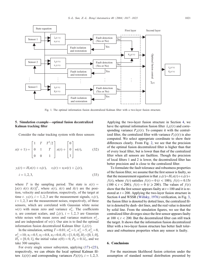
di8erences clearly. From Fig. 2, we see that the precision
of the optimal fusion decentralized !lter is higher than that
of every local !lter, but is lower than that of the centralized
!lter when all sensors are faultless. Though the precision
of local !lters 1 and 2 is lower, the decentralized !lter has
better precision and is close to the centralized !lter.
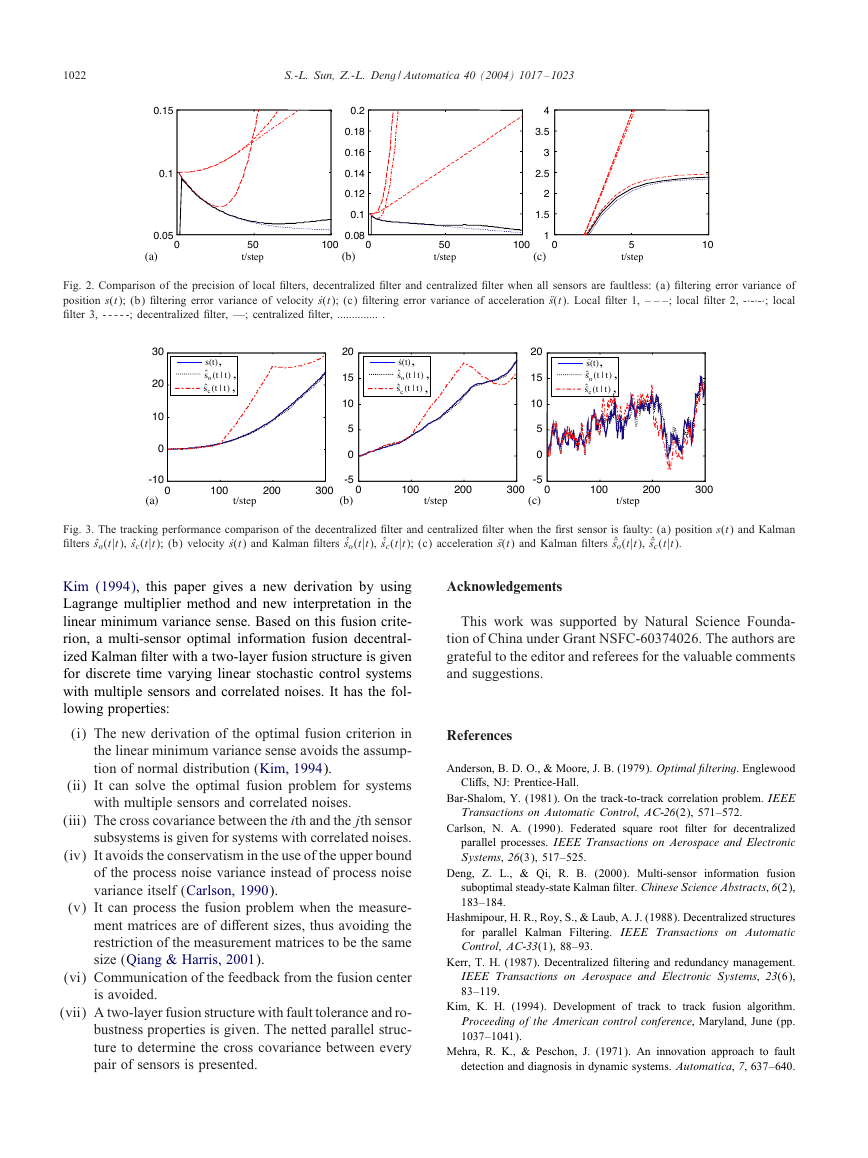
To formulate the fault tolerance and robustness properties
of the fusion !lter, we assume that the !rst sensor is faulty, so
that the measurement equation is that y1(t)=H1x(t)+v1(t)+
f(t), where f(t) satis!es f(t) = 0 (t ¡ 100); f(t) = 0:15t
(100 6 t ¡ 200); f(t) = 0 (t ¿ 200). The values of f(t)
show that the !rst sensor appears faulty at t=100 and it is re-
stored at t = 200. Applying the two-layer fusion structure in
Section 4 and WSSR (Willsky, 1976) veri!cation, in Fig. 3,
the fusion !lter is denoted by dotted lines, the centralized !l-
ter is denoted by dash–dot lines, and the real value is denoted
by solid line. From the simulation !gures, we see that the
centralized !lter diverges since the !rst sensor appears faulty
at 100 6 t ¡ 200. But the decentralized !lter can still track
the target. It shows that the information fusion decentralized
!lter with a two-layer fusion structure has better fault toler-
ance and robustness properties when any sensor is faulty.
6. Conclusions
For every single sensor subsystem, applying (17)–(23),
respectively, we can obtain the local optimal Kalman !l-
ters ˆxi(t|t) and corresponding variances Pi(t|t), i = 1; 2; 3.
For the maximum likelihood fusion criterion under the
assumption of standard normal distribution presented by
�
1022
S.-L. Sun, Z.-L. Deng / Automatica 40 (2004) 1017 – 1023
0.15
0.1
0.05
(a)
0
0.2
0.18
0.16
0.14
0.12
0.1
0.08
(b)
0
4
3.5
3
2.5
2
1.5
1
(c)
0
50
t/step
100
50
t/step
100
5
t/step
10
Fig. 2. Comparison of the precision of local !lters, decentralized !lter and centralized !lter when all sensors are faultless: (a) !ltering error variance of
position s(t); (b) !ltering error variance of velocity ˙s(t); (c) !ltering error variance of acceleration Ts(t). Local !lter 1, – – –; local !lter 2, -·-·-·; local
!lter 3, - - - - -; decentralized !lter, —; centralized !lter, .............. .
s(t),
,
)|(ˆ
t
so
t
,)|(ˆ
sc
t
t
30
20
10
0
s(t),
.
,
.
)|(ˆ
so
t
t
,)|(ˆ
.
t
sc
t
20
15
10
5
0
s(t),
..
,
..
)|(ˆ
so
t
t
,)|(ˆ
..
t
sc
t
20
15
10
5
0
-10
(a)
0
100
t/step
200
300
-5
(b)
0
100
t/step
200
300
-5
(c)
0
100
t/step
200
300
Fig. 3. The tracking performance comparison of the decentralized !lter and centralized !lter when the !rst sensor is faulty: (a) position s(t) and Kalman
!lters ˆso(t|t), ˆsc(t|t); (b) velocity ˙s(t) and Kalman !lters ˆ˙so(t|t), ˆ˙sc(t|t); (c) acceleration Ts(t) and Kalman !lters ˆTso(t|t), ˆTsc(t|t).
Kim (1994), this paper gives a new derivation by using
Lagrange multiplier method and new interpretation in the
linear minimum variance sense. Based on this fusion crite-
rion, a multi-sensor optimal information fusion decentral-
ized Kalman !lter with a two-layer fusion structure is given
for discrete time varying linear stochastic control systems
with multiple sensors and correlated noises. It has the fol-
lowing properties:
(i) The new derivation of the optimal fusion criterion in
the linear minimum variance sense avoids the assump-
tion of normal distribution (Kim, 1994).
(ii) It can solve the optimal fusion problem for systems
with multiple sensors and correlated noises.
(iii) The cross covariance between the ith and the jth sensor
subsystems is given for systems with correlated noises.
(iv) It avoids the conservatism in the use of the upper bound
of the process noise variance instead of process noise
variance itself (Carlson, 1990).
(v) It can process the fusion problem when the measure-
ment matrices are of di8erent sizes, thus avoiding the
restriction of the measurement matrices to be the same
size (Qiang & Harris, 2001).
(vi) Communication of the feedback from the fusion center
is avoided.
(vii) A two-layer fusion structure with fault tolerance and ro-
bustness properties is given. The netted parallel struc-
ture to determine the cross covariance between every
pair of sensors is presented.
Acknowledgements
This work was supported by Natural Science Founda-
tion of China under Grant NSFC-60374026. The authors are
grateful to the editor and referees for the valuable comments
and suggestions.
References
Anderson, B. D. O., & Moore, J. B. (1979). Optimal 9ltering. Englewood
Cli8s, NJ: Prentice-Hall.
Bar-Shalom, Y. (1981). On the track-to-track correlation problem. IEEE
Transactions on Automatic Control, AC-26(2), 571–572.
Carlson, N. A. (1990). Federated square root !lter for decentralized
parallel processes. IEEE Transactions on Aerospace and Electronic
Systems, 26(3), 517–525.
Deng, Z. L., & Qi, R. B. (2000). Multi-sensor information fusion
suboptimal steady-state Kalman !lter. Chinese Science Abstracts, 6(2),
183–184.
Hashmipour, H. R., Roy, S., & Laub, A. J. (1988). Decentralized structures
for parallel Kalman Filtering. IEEE Transactions on Automatic
Control, AC-33(1), 88–93.
Kerr, T. H. (1987). Decentralized !ltering and redundancy management.
IEEE Transactions on Aerospace and Electronic Systems, 23(6),
83–119.
Kim, K. H. (1994). Development of track to track fusion algorithm.
Proceeding of the American control conference, Maryland, June (pp.
1037–1041).
Mehra, R. K., & Peschon, J. (1971). An innovation approach to fault
detection and diagnosis in dynamic systems. Automatica, 7, 637–640.
�
S.-L. Sun, Z.-L. Deng / Automatica 40 (2004) 1017 – 1023
1023
Qiang, G., & Harris, C. J. (2001). Comparison of two measurement
fusion methods for Kalman-!lter-based multisensor data fusion. IEEE
Transactions on Aerospace and Electronic Systems, 37(1), 273–280.
Roy, S., & Iltis, R. A. (1991). Decentralized linear estimation in correlated
measurement noise. IEEE Transactions on Aerospace and Electronic
Systems, 27(6), 939–941.
Saha, R. K. (1996). Track to track fusion with dissimilar sensors.
IEEE Transactions on Aerospace and Electronic Systems, 32(3),
1021–1029.
Saha, R. K. (1998). An eVcient algorithm for multisensor track fusion.
IEEE Transactions on Aerospace and Electronic Systems, 34(1),
200–210.
Willner, D., Chang, C. B., & Dunn, K. P. (1976). Kalman !lter algorithm
for a multisensor system. In Proceedings of IEEE conference on
decision and control, Clearwater, Florida, Dec. (pp. 570–574).
Willsky, A. S. (1976). A survey of design method for failure detection
in dynamic systems. Automatica, 12, 601–611.
Xu, N. S. (2001). Stochastic signal estimation and system control.
Beijing: Beijing Industry University Press.
Shu-Li Sun was born in Heilongjiang,
China in 1971. He received his B.Sc. degree
in department of mathematics and M.Sc.
degree in department of automation from
Heilongjiang University in 1996 and 1999,
respectively. From 1999, he worked as a
faculty member at Heilongjiang University.
Currently he is working for his Ph.D. in
Harbin Institute of Technology. His main
research interests are state estimation, signal
processing and information fusion.
Zi-Li Deng was born in Heilongjiang, China
in 1938. He graduated in department of
mathematics from Heilongjiang University
in 1962. Currently he worked as a profes-
sor at Heilongjiang University. His main re-
search interests are state estimation, signal
processing and information fusion. He has
published more than 200 papers and 5 books
in these areas.
�






 2023年江西萍乡中考道德与法治真题及答案.doc
 2012年重庆南川中考生物真题及答案.doc
 2013年江西师范大学地理学综合及文艺理论基础考研真题.doc
 2020年四川甘孜小升初语文真题及答案I卷.doc
 2020年注册岩土工程师专业基础考试真题及答案.doc
 2023-2024学年福建省厦门市九年级上学期数学月考试题及答案.doc
 2021-2022学年辽宁省沈阳市大东区九年级上学期语文期末试题及答案.doc
 2022-2023学年北京东城区初三第一学期物理期末试卷及答案.doc
 2018上半年江西教师资格初中地理学科知识与教学能力真题及答案.doc
 2012年河北国家公务员申论考试真题及答案-省级.doc
 2020-2021学年江苏省扬州市江都区邵樊片九年级上学期数学第一次质量检测试题及答案.doc
 2022下半年黑龙江教师资格证中学综合素质真题及答案.doc