线性系统的快速优化与电力系统相关.pdf

发布时间：2022-06-08 发布人：admin 分类：说明书资料大小：2.01M 资料格式：pdf 举报版权申诉

ludaqing-1315385-4744302543450703834.pdf-第1页.png

第1页 / 共13页

ludaqing-1315385-4744302543450703834.pdf-第2页.png

第2页 / 共13页

ludaqing-1315385-4744302543450703834.pdf-第3页.png

第3页 / 共13页

ludaqing-1315385-4744302543450703834.pdf-第4页.png

第4页 / 共13页

ludaqing-1315385-4744302543450703834.pdf-第5页.png

第5页 / 共13页

ludaqing-1315385-4744302543450703834.pdf-第6页.png

第6页 / 共13页

ludaqing-1315385-4744302543450703834.pdf-第7页.png

第7页 / 共13页

ludaqing-1315385-4744302543450703834.pdf-第8页.png

第8页 / 共13页

Article Contents

p. 220

p. 221

p. 222

p. 223

p. 224

p. 225

p. 226

p. 227

p. 228

p. 229

p. 230

p. 231

p. 232

Issue Table of Contents

Operations Research, Vol. 39, No. 2 (Mar. - Apr., 1991), pp. 179-350

Front Matter [pp. 179-179]

In This Issue [pp. 180-182]

OR Forum

An Existence Theorem for OR/MS [pp. 183-193]

OR Practice

The Application of Operations Research in the Optimization of Agricultural Production [pp. 194-205]

Decision Analysis Applications in the Operations Research Literature, 1970-1989 [pp. 206-219]

A Rapid Method for Optimization of Linear Systems with Storage [pp. 220-232]

Multi-Item Replenishment and Storage Problem (MIRSP): Heuristics and Bounds [pp. 233-243]

Some Facets for an Assignment Problem with Side Constraints [pp. 244-250]

Interpolation Approximations, of Sojourn Time Distributions [pp. 251-260]

Optimal Scheduling of Inspections: A Delayed Markov Model with False Positives and Negatives [pp. 261-273]

A Secretary Problem with Uncertain Employment and Best Choice of Available Candidates [pp. 274-284]

Minimax Resource Allocation with Tree Structured Substitutable Resources [pp. 285-295]

Simultaneous Product-Mix Planning, Lot Sizing and Scheduling at Bottleneck Facilities [pp. 296-307]

An (S - 1, S) Inventory System with Emergency Orders [pp. 308-321]

Brownian Networks with Discretionary Routing [pp. 322-340]

Optimal Data Verification Tests [pp. 341-348]

Back Matter [pp. 349-350]

A RAPID METHOD FOR OPTIMIZATION OF LINEAR SYSTEMS WITH STORAGE Intelligent Energy Systems Ltd., Crows Nest, New South Wales, Australia C. H. BANNISTER R. J. KAYE University of New South Wales, Kensington, New South Wales, Australia (Received March 1989; revision received January 1990; accepted January 1990) A new method for optimizing the operation of a single storage connected to a general linear memoryless system is presented. The model is shown to cover a wide variety of practical situations where a deterministic approximation is valid. The method combines linear and dynamic programming concepts to produce a fast but exact optimization. Storage devices can be used for commodities with costs or availabilities that change with time. Eco- nomic benefits are gained by storing the commodity when * its cost is low, or * demand for it is low for use at other times when * the cost is higher, or * it is in demand. For example, storage is commonly used in large-scale power systems in the form of dams with generation and pumping facilities, in small-scale remote area power supply systems (batteries) and in many types of industrial and commercial activities. The systems considered in this paper consist of a single store and a production facility. In the case of an electric power system, the production facility consists of the model of, inter alia, the generating units, the loads and dam spillages and inflows. In the absence of storage, the thermal generation units are dispatched using the merit order rule: the units are loaded in increasing order of variable cost until the demand is satisfied. Storage significantly complicates this process because it links operations between time periods, so that optimization of operations cannot be carried out independently in each time period. In this paper, a new exact optimization technique is presented. Combining linear programming and dynamic programming concepts, the technique optimizes the op- eration of the storage by solving a sequence of small linear programming problems rather than the much larger, time-staged problem. By exploiting specific fea- tures of the single-stage problem, a very rapid solution method has been devised. A number of mathematical methods have been applied to the operational optimization problem, including dy- namic programming (Lukic 1982), the maximum princi- ple of optimal control (Martin and Dillon 1977) and linear, nonlinear and mixed integer programming (Meliopoulos and Skordilis 1979, Halliburton and Sirisena 1982, Habibollahzadeh and Bubenko 1986). However, the applicability of these methods to practical problems has been limited by their computational bur- den. For example, the number of constraints in a simple linear programming formulation of a storage optimiza- tion will be proportional to the number of time steps. Solution time will vary approximately as the cube of the number of time steps. This places a relatively small practical limit on the size and duration of problems that can be solved. Dechamps, Nuytten and Lee (1980) derived the Kuhn-Tucker necessary conditions for the solution of a particular deterministic single storage problem. These conditions were then used to develop a heuristic solution Subject classifications: Dynamic programming, deterministic: rapid, exact dynamic programming. Production/scheduling: optimal utilization of storage. Programming, linear: fast optimization of linear systems. Operations Research Vol. 39, No. 2, March-April 1991 220 0030-364X/9 1/3902-0220 $01.25 (D 1991 Operations Research Society of America

method, avoiding the need to solve the very large linear program directly. The method was reported to be some ten times faster than a dynamic programming approach. However, the solutions exhibited some departure from optimality, presumably because the heuristics did not lead to the Kuhn-Tucker conditions being satisfied exactly. In the work of Daryanian (1986), the optimization ofthe operation of a simple production process with stor- age was formulated as a time-sequenced network. A spe- cial purpose solution procedure for this problem was developed and tested. It performed much faster than a standard simplex routine. However, this algorithm can- not handle complex production facilities that exhibit time-variation in the inputs, outputs, production pro- cesses or costs. 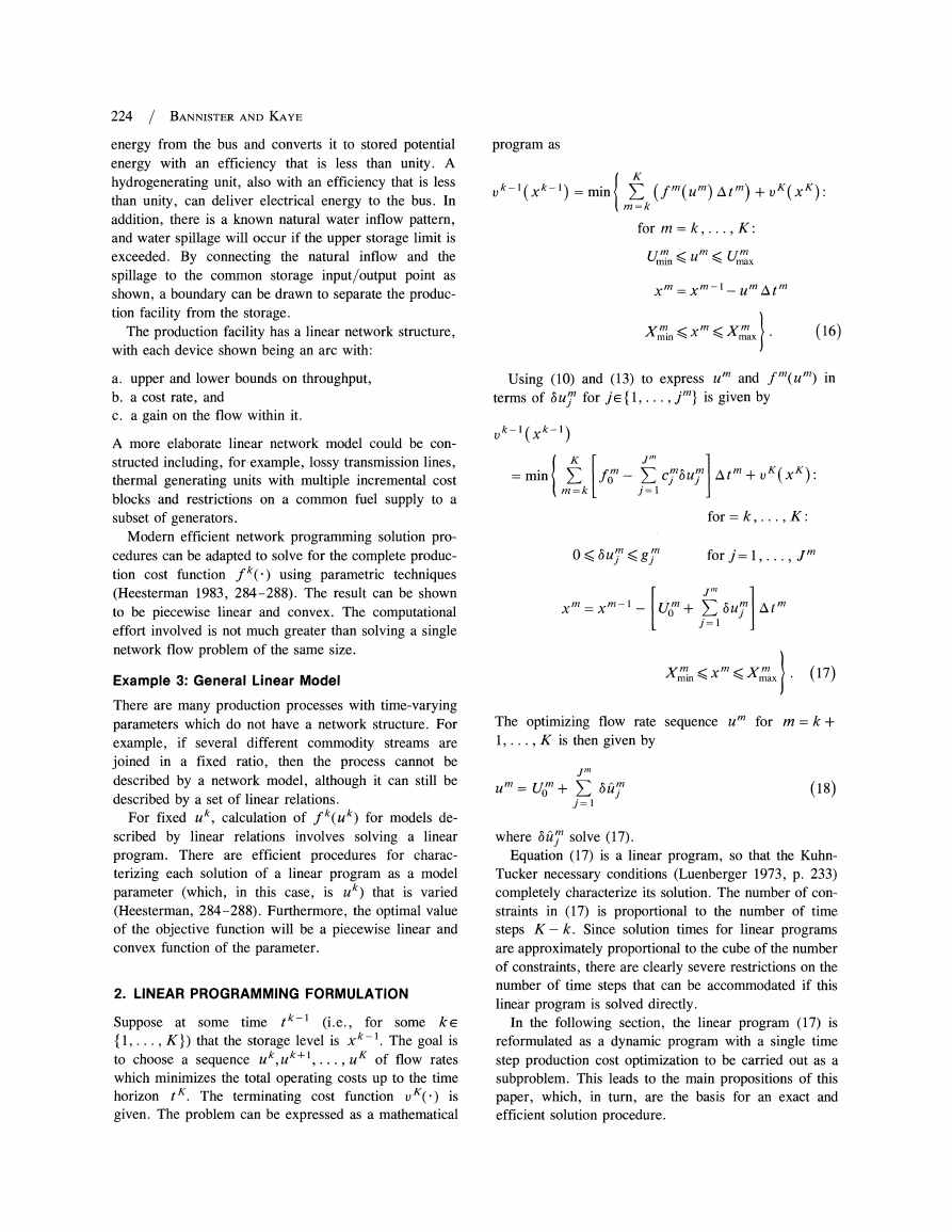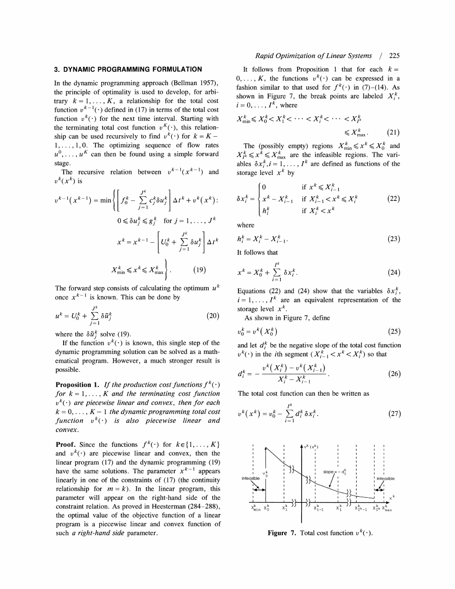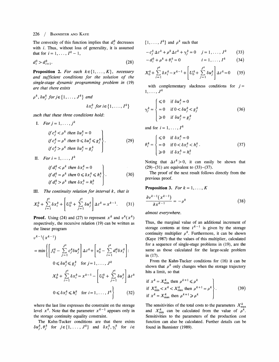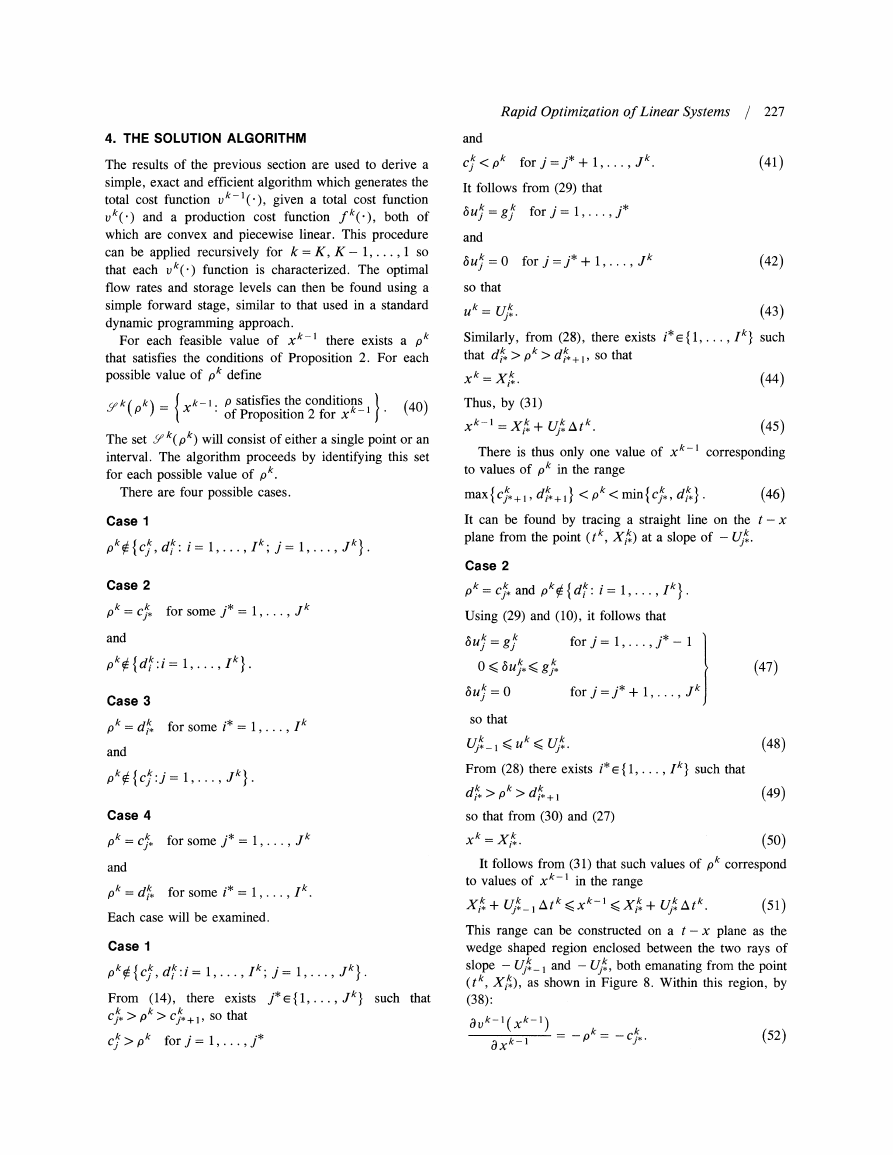In this paper, we present a new, efficient and exact method for solving a very general class of deterministic problems with a single storage. In Section 1, the model of systems to be optimized is described. It consists of a single storage and a production facility, which is de- scribed by a piecewise linear production cost function. This function is constant within a number of time inter- vals that make up the study period. Some examples, also presented in Section 1, illustrate how this model can be used to describe a wide range of industrial situations. One contribution of this paper is the recognition that the modeling of the production facility and the optimization of the storage operation can be separated. In Section 2, the storage optimization problem is formulated as a linear program. This formulation is used in Section 3 to derive certain general properties of the optimal solution which, therefore, also apply to the dynamic programming solution. Key among these is the central role played by the Kuhn-Tucker multiplier asso- ciated with the continuity equation, which describes the operation of the storage. This multiplier can be shown to equal the incremental value of commodity in the storage. These properties are exploited in Section 4 to develop the solution method, which amounts to solving a small linear program at each time step. However, by further exploiting the special properties of the problem, a solu- tion technique that is much faster than the simplex method has been developed. In Sections 5 and 6, illustra- tive examples are detailed and discussed. The procedure gives exact results because it systemati- cally and explicitly satisfies the Kuhn-Tucker necessary and sufficient conditions for the solution of the linear program. Although the method uses dynamic program- ming concepts, no discretization of the storage space is required, thus avoiding the usual approximations associ- ated with dynamic programming. Rapid Optimization of Linear Systems / 221 1. SYSTEM DESCRIPTION 1.1. 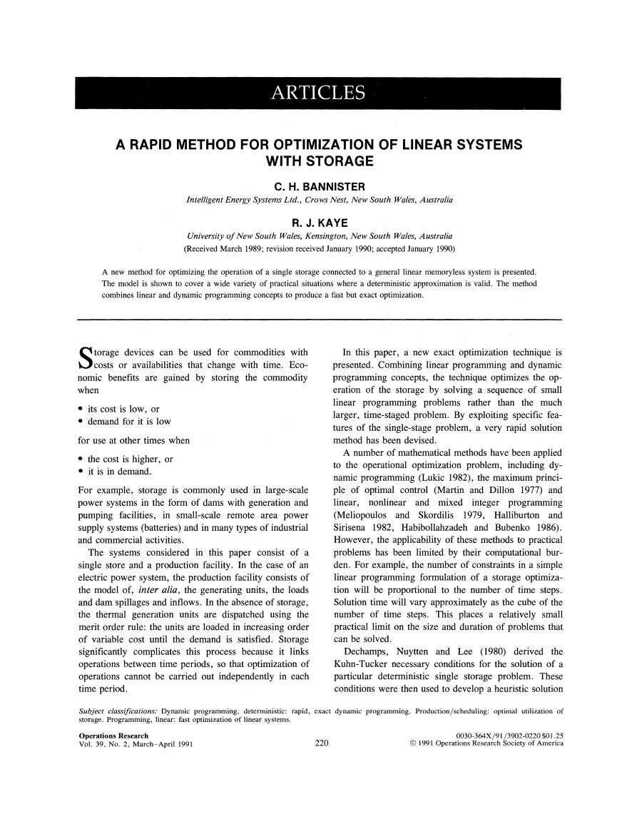The Production and Storage Model The system whose operation is to be optimized consists of two components: a storage and a general, memoryless production facility which feeds material into and out of the storage, as shown in Figure 1. The time period under study, to < t < T, is partitioned into K time intervals. It is assumed that the flow rate of material, the state of the production facility and the constraints on the amount of storage are constant over each interval. Thus, if the time points that partition the period under study are t1 < . . . < tk < t 0< then for k = 1, ... 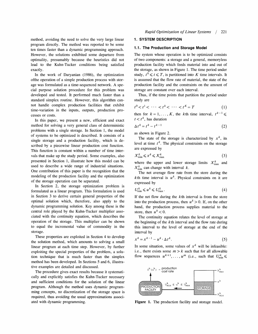t < tk', has duration < tK= T , K, the kth time interval, tk-l < k-i 'A tk = t k- as shown in Figure 2. (2) The state of the storage is characterized by x k, its level at time tk. The physical constraints on the storage are expressed by Xk. Xk < Xax (3) where the upper and lower storage limits Xmk and min can change with interval k. The net average flow rate from the store during the kth time interval is uk. Physical constraints on it are expressed by Umax. (4) Umk~l? 0. If, on the other hand, the production process supplies material to the store, then uk< O. The continuity equation relates the level of storage at the beginning of the kth interval and the flow rate during this interval to the level of storage at the end of the interval by k-i - Uk.5Atk) Xk = In some situation, some values of x k will be infeasible: i.e., there exists some m > k such that for all allowable flow sequences uk+1,... (i.e., such that Ut in? , U f fk(Uk) = production cost ratema u Um < k < Uk max RODUCTION< FACILITY Figure 1. The production facility and storage Xka k modlin Figure 1. The production facility and storage model.

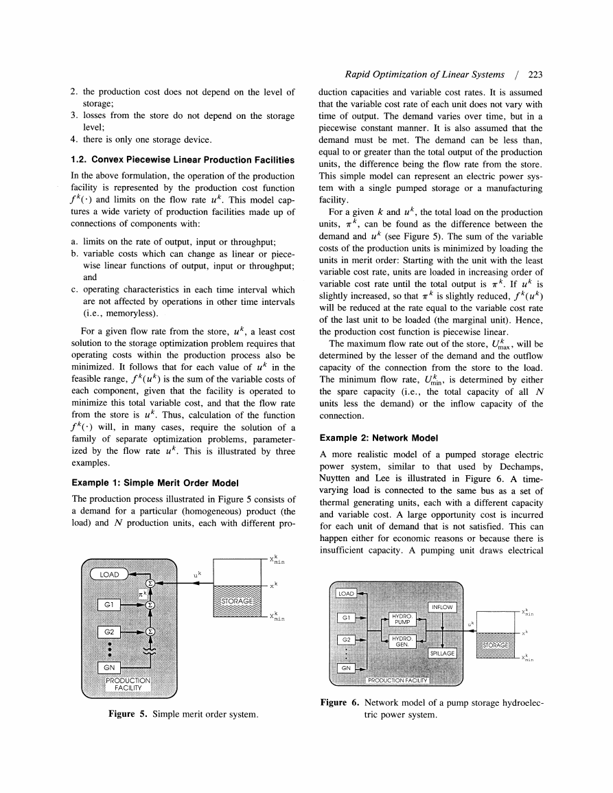
222 / BANNISTER AND KAYE At At k At time,t 0 U3 Uk U a2 u~ 1 u~ u~1 ~k U t? t 1 tk- tk tK tK T k k - k k k k k k kth interval Figure 2. Partition of the time period into K intervals. 1< 6k =03- k k 6Tu3k=IO Figure 4. Definition of 6 ujk flow ~~~~~~~~rate for n = k + 1, . , m), the level of storage at Un Um time tm obtained by repeated application of (5), xm, will not obey the storage level limits (3), either xm > Xmax or xm < Xmn. (6) If the net flow rate from the storage during the kth interval is uk, then the net cost per unit time incurred in the production facility is denoted as f k(Uk). Note that f k(Uk) can be negative, denoting a net profit. The total net production cost during the kth interval is f k(Uk)A tk. In this paper, it is assumed that for each interval k = 1, . . . 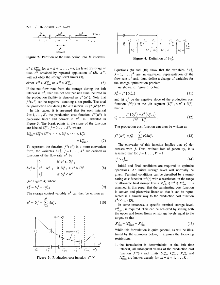, K, the production cost function fk(uk) is piecewise linear and convex in uk, as illustrated in Figure 3. The break points in the slope of the function are labeled Uk, j= 0,. . . , jk, where Uk=wk< Ulk< ... < U < ... < U~k = Uk. (7) To represent the function f k(Uk) in a more convenient jk are defined as form, the variables 6uj/, ]=1,..., functions of the flow rate uk by r Uk Uk-Uk gk if Uk< Y/?-i if U1 < Uk< Uk if Uk < uk (8) (see Figure 4) where gI%41k Uk1 (9) The storage control variable uk can then be written as jk U Uok + E u$.k(10) j=1 ,Ki fk (uk) I I I fk siope C i L: X ,L Figure 3. Production cost function f k( *). Equations (8) and (10) show that the variables 6uk jk are an equivalent representation of the J = 1,..., flow rate uk and, thus, define a change of variables for the storage optimization problem. As shown in Figure 3, define fk fk(Uk) (11) and let function fk(.) that is be the negative slope of the production cost in the jth segment (Uj k Cy+1 (14) Initial and final conditions are required to optimize operations. An initial storage level will normally be given. Terminal conditions can be described by a termi- nating cost function v K(.) with a restriction on the range of allowable final storage levels X4i < x < XK . It is assumed in this paper that the terminating cost function is convex and piecewise linear so that it can be repre- sented in a similar way to the production cost function fk(.) in (13). In some instances, a specific terminal storage level, XtaKrget is required. This can be achieved by setting both the upper and lower limits on storage levels equal to the target, so that Xm target Xmax,*(1 While this formulation is quite general, as will be illus- trated by the examples below, it imposes the following restrictions: 1. the formulation is deterministic: at the kth time interval, all subsequent values of the production cost function fm(*) and limits Umin Ummx, Xmin and Xmax are known exactly for m = k + 1, ... ., K;

2. the production cost does not depend on the level of storage; 3. losses from the store do not depend on the storage level; 4. there is only one storage device. 1.2. Convex Piecewise Linear Production Facilities In the above formulation, the operation of the production facility is represented by the production cost function and limits on the flow rate Uk. This model cap- fk(.) tures a wide variety of production facilities made up of connections of components with: a. limits on the rate of output, input or throughput; b. variable costs which can change as linear or piece- wise linear functions of output, input or throughput; and c. operating characteristics in each time interval which are not affected by operations in other time intervals (i.e., memoryless). For a given flow rate from the store, u k, a least cost solution to the storage optimization problem requires that operating costs within the production process also be minimized. It follows that for each value of uk in the feasible range, f k(Uk) is the sum of the variable costs of each component, given that the facility is operated to minimize this total variable cost, and that the flow rate from the store is uk. Thus, calculation of the function f k(.) will, in many cases, require the solution of a family of separate optimization problems, parameter- ized by the flow rate uk. This is illustrated by three examples. Example 1: Simple Merit Order Model The production process illustrated in Figure 5 consists of a demand for a particular (homogeneous) product (the load) and N production units, each with different pro- LOAD .. >;t~~~~~o? UkXk~~~~in U k Rapid Optimization of Linear Systems / 223 duction capacities and variable cost rates. It is assumed that the variable cost rate of each unit does not vary with time of output. The demand varies over time, but in a piecewise constant manner. It is also assumed that the demand must be met. The demand can be less than, equal to or greater than the total output of the production units, the difference being the flow rate from the store. This simple model can represent an electric power sys- tem with a single pumped storage or a manufacturing facility. For a given k and uk, the total load on the production units, r k, can be found as the difference between the demand and u k (see Figure 5). The sum of the variable costs of the production units is minimized by loading the units in merit order: Starting with the unit with the least variable cost rate, units are loaded in increasing order of variable cost rate until the total output is k. If U k is slightly increased, so that 7rk is slightly reduced, f k(Uk) will be reduced at the rate equal to the variable cost rate of the last unit to be loaded (the marginal unit). Hence, the production cost function is piecewise linear. The maximum flow rate out of the store, Uk , will be determined by the lesser of the demand and the outflow capacity of the connection from the store to the load. The minimum flow rate, Uk. , is determined by either the spare capacity (i.e., the total capacity of all N units less the demand) or the inflow capacity of the connection. Example 2: Network Model A more realistic model of a pumped storage electric power system, similar to that used by Dechamps, Nuytten and Lee is illustrated in Figure 6. A time- varying load is connected to the same bus as a set of thermal generating units, each with a different capacity and variable cost. A large opportunity cost is incurred for each unit of demand that is not satisfied. This can happen either for economic reasons or because there is insufficient capacity. A pumping unit draws electrical Gi ~~~~~~STORAG ll1 0 1 1 - X k~~~~~~~~~in GN PRODUCTION ~~~~~~~~~~~~~~.s.. e S. .... ...... FACIL . o s INFLOW k HmDR PUM l k HYDRO GEN.SORG ~~~~~~~~~~~~~~~~Xk Figure 5. Simple merit order system. Figure 6. Network model of a pump storage hydroelec- tric power system.

224 / BANNISTER AND KAYE energy from the bus and converts it to stored potential energy with an efficiency that is less than unity. A hydrogenerating unit, also with an efficiency that is less than unity, can deliver electrical energy to the bus. In addition, there is a known natural water inflow pattern, and water spillage will occur if the upper storage limit is exceeded. By connecting the natural inflow and the spillage to the common storage input/output point as shown, a boundary can be drawn to separate the produc- tion facility from the storage. The production facility has a linear network structure, with each device shown being an arc with: a. upper and lower bounds on throughput, b. a cost rate, and c. a gain on the flow within it. A more elaborate linear network model could be con- structed including, for example, lossy transmission lines, thermal generating units with multiple incremental cost blocks and restrictions on a common fuel supply to a subset of generators. Modern efficient network programming solution pro- cedures can be adapted to solve for the complete produc- tion cost function f k(*) using parametric techniques (Heesterman 1983, 284-288). The result can be shown to be piecewise linear and convex. The computational effort involved is not much greater than solving a single network flow problem of the same size. Example 3: General Linear Model There are many production processes with time-varying parameters which do not have a network structure. For example, if several different commodity streams are joined in a fixed ratio, then the process cannot be described by a network model, although it can still be described by a set of linear relations. For fixed uk, calculation of fk(Uk) for models de- scribed by linear relations involves solving a linear program. There are efficient procedures for charac- terizing each solution of a linear program as a model parameter (which, in this case, is uk) that is varied (Heesterman, 284-288). Furthermore, the optimal value of the objective function will be a piecewise linear and convex function of the parameter. 2. LINEAR PROGRAMMING FORMULATION tk-1 (i.e., Suppose at some time for some ke {1, ... , K }) that the storage level is Xk- 1. The goal is to choose a sequence uk, Uk+1, ..., uK of flow rates which minimizes the total operating costs up to the time horizon t K. The terminating cost function v K(.) is given. The problem can be expressed as a mathematical program as vk-l(Xk-i) K = min{ E m =k (fm(um) Atm) + vK(xK): for m =k ... , K: .m =Xml_ UmAtm XmM. < M < XmaX}. (16) Using (10) and (13) to express um and fm(um) in terms of 6uT for je ,. ., jm} is given by Vk- k ( X ) = minm { 1 K m=k L im - E CJ6ul Attm + VK(XK) j= I for = k, ... I K: 0 <' 6U

3. DYNAMIC PROGRAMMING FORMULATION In the dynamic programming approach (Bellman 1957), the principle of optimality is used to develop, for arbi- trary k = 1, . . . , K, a relationship for the total cost function v k- 1( * ) defined in (17) in terms of the total cost for the next time interval. Starting with function v k(.) the terminating total cost function vK(. ), this relation- ship can be used recursively to find v k(.) 1,... uo, ... stage. ,1,0. The optimizing sequence of flow rates , uK can then be found using a simple forward for k = K - The recursive relation between v k-i (xk- ) and V k(Xk) is k-1(Xk-1) min f f gk1 k E Cj6U1 j=l tk+vk(Xk) 0 < 6u gj for j = 1, Jk XmiIn

/ BANNISTER AND KAYE 226 The convexity of this function implies that d4 decreases with i. Thus, without loss of generality, it is assumed that for E- k_ 1, 1'. . di > d+1. Proposition 2. For each ke { 1,... , K}, necessary and sufficient conditions for the solution of the single-stage dynamic programming problem in (19) are that there exists (28) pka uforje{1 ,Jk} and < forie{1, ...Ik} such that these three conditions hold: I. Forj= 1,..., jk 0 if Ck < pk then W u if c _=pk thenO?u>,g pk then 6 g {I. ..Ik} and Pk such that -_ci Atk' +pkAtk+ ykz=O j= 1 jk dik+ pk+Gk=O i= 1, ... Itk xt+? E a-X_Xk- i~~~~l~ IkrJkl + Iuok+Z j=l I kAtk=o (33) (34) (35) with complementary slackness conditions for j 1,.,, j ok and for i1, .. .>I (29) ok ' 40 if ax> =O =o o if O<6x if xk =hk H (37) II. For i = 1, ...,Ik if di < pk then Wx -? if d _=pk then O < if dc > pk then x = h h Ci[fu J l jo jk Atk+ Vk 0 6u< gj for j= 1, i= 1 d x k1 - Jk Zi O yok 6X ai= I Xk-1 0 Uok+ 6Uk 1: - 1 A t 0 < bx < h for i= 1,...Ik (32) where the last line expresses the constraint on the storage level xk. Note that the parameter x k-1 appears only in the storage continuity equality constraint. The Kuhn-Tucker conditions are that there exists , for ie 8uk, G for je{1 .., J'} and Noting that A t k> 0, it can easily be shown that (29)-(31) are equivalent to (33)-(37). The proof of the next result follows directly from the previous proof. Proposition. Fork=1,...,K dvk1(xkl) k almost everywhere. (38) Thus, the marginal value of an additional increment of is given by the storage storage contents at time tkil continuity multiplier pk. Furthermore, it can be shown (Kaye 1987) that the values of this multiplier, calculated for a sequence of single-stage problems in (19) are the same as those calculated for the large-scale problem in (17). From the Kuhn-Tucker conditions for (16) it can be shown that ji' only changes when the storage trajectory hits a limit, so that if xkI=X a ek+e then pk+1 pk (39) The sensitivities of the total costs to the parameters Xtax and Xmm can be calculated from the value of pk Sensitivities to the parameters of the production cost function can also be calculated. Further details can be found in Bannister (1989).

4. THE SOLUTION ALGORITHM The results of the previous section are used to derive a simple, exact and efficient algorithm which generates the total cost function vk-i (), given a total cost function Vk( ) and a production cost function f k(. ), both of which are convex and piecewise linear. This procedure can be applied recursively for k = K, K - 1, ... , 1 so that each vk( ) function is characterized. The optimal flow rates and storage levels can then be found using a simple forward stage, similar to that used in a standard dynamic programming approach. For each feasible value of xk-1 there exists a p k that satisfies the conditions of Proposition 2. For each possible value of pk define k( P k)= x k-i. p satisfies theconditions of Proposition 2for x i kI , ) 40) The set 92 k( pk) will consist of either a single point or an interval. The algorithm proceeds by identifying this set for each possible value of pk. There are four possible cases. Case 1 pko ? C, dik: i = I, ..ik j I j k} Case 2 pk =C * for some j*=1, Jk and pk {d IC: l Ik} Case 3 p =di* for somei*=1,...,I and pk {ck:j = , ...,Jk}. Case 4 pk =Cj/* for some j* =1.Jk and for some i* = 1,. . .,. I. p =di* Each case will be examined. Case 1 c, dik:i = II . .. pko ? From (14), there exists j*e{1, k c1 > P > c1* +, so that Iik; j= k k I jk} . . ., jk} such that Rapid Optimization of Linear Systems / 227 and C1 < p k k 1 for j =j* + 1, . j Jk (41) It follows from (29) that bUk = gj for j = 1, j* and bu = O forj=j*+1,..., jk so that uk= Ukj*. Similarly, from (28), there exists i* E{ 1,.. that di >pk> xk=X Thus, by (31) so that d*+, . Xk1 = Xk*+ Uj Atk. (42) (43) , I'k} such (44) (45) There is thus only one value of x k-i corresponding to values of pk in the range max cj*+1,c4+1} di*+ 1 From (28) there exists i*e{1, di* > so that from (30) and (27) xk =X. . ., I'} such that (48) (49) (50) It follows from (31) that such values of pk correspond X TufA tk. to values of x k-1 in the range + X/k+ U)k Atk xkl? (51) This range can be constructed on a t - x plane as the wedge shaped region enclosed between the two rays of slope - and - U'T, both emanating from the point (tk, X/*), as shown in Figure 8. Within this region, by (38): a Vk_ __ j1 1 ) ( k - p _ k -c1*. x (52)

分享到：

赞收藏

资料库

线性系统的快速优化与电力系统相关.pdf

相关推荐

课程资源

热门标签

最新资料