Stochastic Calculus for Finance, Volume I and II
Solution of Exercise Problems
Yan Zeng
August 20, 2007
�
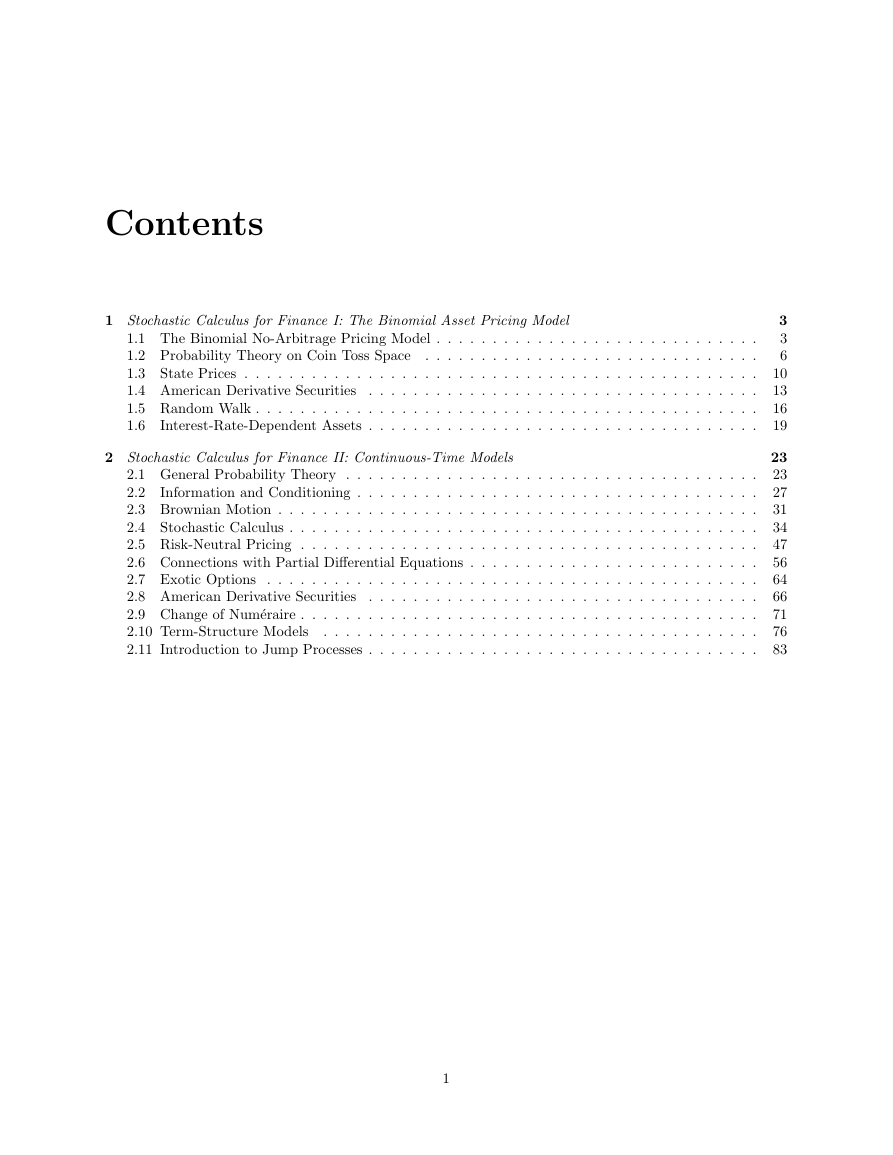
Contents
1 Stochastic Calculus for Finance I: The Binomial Asset Pricing Model
1.1 The Binomial No-Arbitrage Pricing Model . . . . . . . . . . . . . . . . . . . . . . . . . . . . .
1.2 Probability Theory on Coin Toss Space
. . . . . . . . . . . . . . . . . . . . . . . . . . . . . .
1.3 State Prices . . . . . . . . . . . . . . . . . . . . . . . . . . . . . . . . . . . . . . . . . . . . . .
1.4 American Derivative Securities
. . . . . . . . . . . . . . . . . . . . . . . . . . . . . . . . . . .
1.5 Random Walk . . . . . . . . . . . . . . . . . . . . . . . . . . . . . . . . . . . . . . . . . . . . .
Interest-Rate-Dependent Assets . . . . . . . . . . . . . . . . . . . . . . . . . . . . . . . . . . .
1.6
2 Stochastic Calculus for Finance II: Continuous-Time Models
2.1 General Probability Theory . . . . . . . . . . . . . . . . . . . . . . . . . . . . . . . . . . . . .
2.2
Information and Conditioning . . . . . . . . . . . . . . . . . . . . . . . . . . . . . . . . . . . .
2.3 Brownian Motion . . . . . . . . . . . . . . . . . . . . . . . . . . . . . . . . . . . . . . . . . . .
2.4 Stochastic Calculus . . . . . . . . . . . . . . . . . . . . . . . . . . . . . . . . . . . . . . . . . .
2.5 Risk-Neutral Pricing . . . . . . . . . . . . . . . . . . . . . . . . . . . . . . . . . . . . . . . . .
2.6 Connections with Partial Differential Equations . . . . . . . . . . . . . . . . . . . . . . . . . .
2.7 Exotic Options . . . . . . . . . . . . . . . . . . . . . . . . . . . . . . . . . . . . . . . . . . . .
2.8 American Derivative Securities
. . . . . . . . . . . . . . . . . . . . . . . . . . . . . . . . . . .
2.9 Change of Num´eraire . . . . . . . . . . . . . . . . . . . . . . . . . . . . . . . . . . . . . . . . .
2.10 Term-Structure Models
. . . . . . . . . . . . . . . . . . . . . . . . . . . . . . . . . . . . . . .
2.11 Introduction to Jump Processes . . . . . . . . . . . . . . . . . . . . . . . . . . . . . . . . . . .
3
3
6
10
13
16
19
23
23
27
31
34
47
56
64
66
71
76
83
1
�
This is a solution manual for the two-volume textbook Stochastic calculus for finance, by Steven Shreve.
If you have any comments or find any typos/errors, please email me at yz44@cornell.edu.
The current version omits the following problems. Volume I: 1.5, 3.3, 3.4, 5.7; Volume II: 3.9, 7.1, 7.2,
7.5–7.9, 10.8, 10.9, 10.10.
Acknowledgment I thank Hua Li (a graduate student at Brown University) for reading through this
solution manual and communicating to me several mistakes/typos. I also thank Hideki Murakami for pointing
out a typo in Exercise 4.3, Volume II.
2
�
Chapter 1
Stochastic Calculus for Finance I: The
Binomial Asset Pricing Model
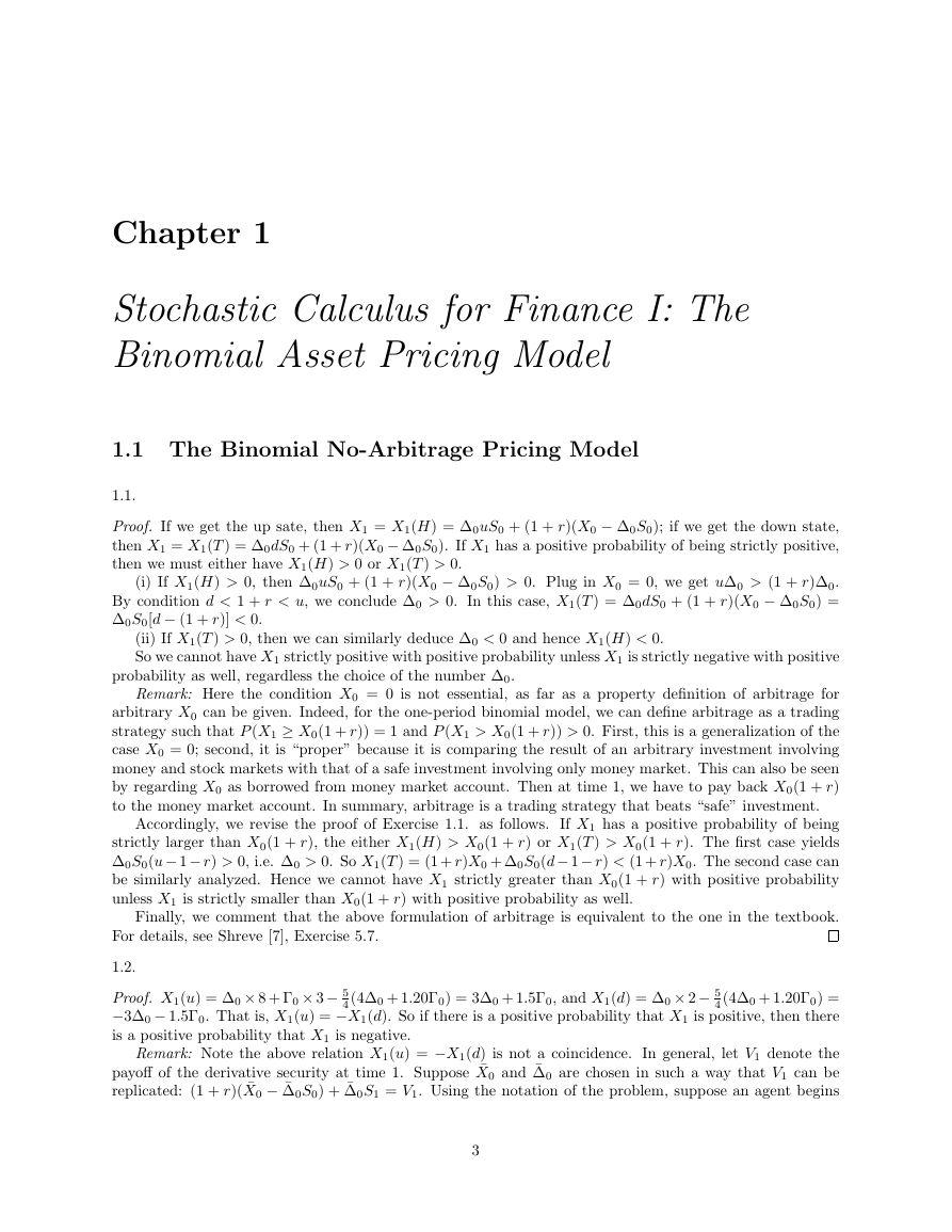
1.1 The Binomial No-Arbitrage Pricing Model
1.1.
Proof. If we get the up sate, then X1 = X1(H) = ∆0uS0 + (1 + r)(X0 − ∆0S0); if we get the down state,
then X1 = X1(T ) = ∆0dS0 + (1 + r)(X0 − ∆0S0). If X1 has a positive probability of being strictly positive,
then we must either have X1(H) > 0 or X1(T ) > 0.
(i) If X1(H) > 0, then ∆0uS0 + (1 + r)(X0 − ∆0S0) > 0. Plug in X0 = 0, we get u∆0 > (1 + r)∆0.
By condition d < 1 + r < u, we conclude ∆0 > 0. In this case, X1(T ) = ∆0dS0 + (1 + r)(X0 − ∆0S0) =
∆0S0[d − (1 + r)] < 0.
(ii) If X1(T ) > 0, then we can similarly deduce ∆0 < 0 and hence X1(H) < 0.
So we cannot have X1 strictly positive with positive probability unless X1 is strictly negative with positive
probability as well, regardless the choice of the number ∆0.
Remark: Here the condition X0 = 0 is not essential, as far as a property definition of arbitrage for
arbitrary X0 can be given. Indeed, for the one-period binomial model, we can define arbitrage as a trading
strategy such that P (X1 ≥ X0(1 + r)) = 1 and P (X1 > X0(1 + r)) > 0. First, this is a generalization of the
case X0 = 0; second, it is “proper” because it is comparing the result of an arbitrary investment involving
money and stock markets with that of a safe investment involving only money market. This can also be seen
by regarding X0 as borrowed from money market account. Then at time 1, we have to pay back X0(1 + r)
to the money market account. In summary, arbitrage is a trading strategy that beats “safe” investment.
Accordingly, we revise the proof of Exercise 1.1. as follows. If X1 has a positive probability of being
strictly larger than X0(1 + r), the either X1(H) > X0(1 + r) or X1(T ) > X0(1 + r). The first case yields
∆0S0(u− 1− r) > 0, i.e. ∆0 > 0. So X1(T ) = (1 + r)X0 + ∆0S0(d− 1− r) < (1 + r)X0. The second case can
be similarly analyzed. Hence we cannot have X1 strictly greater than X0(1 + r) with positive probability
unless X1 is strictly smaller than X0(1 + r) with positive probability as well.
Finally, we comment that the above formulation of arbitrage is equivalent to the one in the textbook.
For details, see Shreve [7], Exercise 5.7.
1.2.
Proof. X1(u) = ∆0 × 8 + Γ0 × 3− 5
4(4∆0 + 1.20Γ0) =
−3∆0 − 1.5Γ0. That is, X1(u) = −X1(d). So if there is a positive probability that X1 is positive, then there
is a positive probability that X1 is negative.
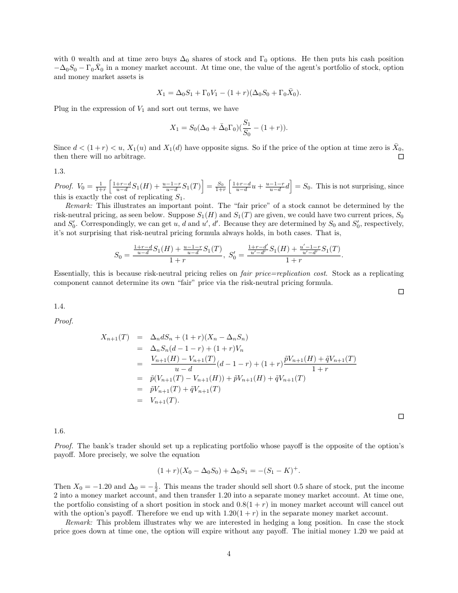
Remark: Note the above relation X1(u) = −X1(d) is not a coincidence. In general, let V1 denote the
payoff of the derivative security at time 1. Suppose ¯X0 and ¯∆0 are chosen in such a way that V1 can be
replicated: (1 + r)( ¯X0 − ¯∆0S0) + ¯∆0S1 = V1. Using the notation of the problem, suppose an agent begins
4(4∆0 + 1.20Γ0) = 3∆0 + 1.5Γ0, and X1(d) = ∆0 × 2− 5
3
�
with 0 wealth and at time zero buys ∆0 shares of stock and Γ0 options. He then puts his cash position
−∆0S0 − Γ0 ¯X0 in a money market account. At time one, the value of the agent’s portfolio of stock, option
and money market assets is
X1 = ∆0S1 + Γ0V1 − (1 + r)(∆0S0 + Γ0 ¯X0).
Plug in the expression of V1 and sort out terms, we have
X1 = S0(∆0 + ¯∆0Γ0)( S1
S0
− (1 + r)).
Since d < (1 + r) < u, X1(u) and X1(d) have opposite signs. So if the price of the option at time zero is ¯X0,
then there will no arbitrage.
1+r−d
= S0
1+r
u−d u + u−1−r
u−d d
= S0. This is not surprising, since
1.3.
1+r−d
u−d S1(H) + u−1−r
Proof. V0 = 1
1+r
this is exactly the cost of replicating S1.
u−d S1(T )
Remark: This illustrates an important point. The “fair price” of a stock cannot be determined by the
risk-neutral pricing, as seen below. Suppose S1(H) and S1(T ) are given, we could have two current prices, S0
and S
0, respectively,
it’s not surprising that risk-neutral pricing formula always holds, in both cases. That is,
0. Correspondingly, we can get u, d and u, d. Because they are determined by S0 and S
S0 =
1+r−d
u−d S1(H) + u−1−r
u−d S1(T )
1 + r
, S
0 =
1+r−d
u−d S1(H) + u−1−r
u−d S1(T )
1 + r
.
Essentially, this is because risk-neutral pricing relies on fair price=replication cost. Stock as a replicating
component cannot determine its own “fair” price via the risk-neutral pricing formula.
1.4.
Proof.
1.6.
Xn+1(T ) = ∆ndSn + (1 + r)(Xn − ∆nSn)
= ∆nSn(d − 1 − r) + (1 + r)Vn
= Vn+1(H) − Vn+1(T )
= ˜p(Vn+1(T ) − Vn+1(H)) + ˜pVn+1(H) + ˜qVn+1(T )
= ˜pVn+1(T ) + ˜qVn+1(T )
= Vn+1(T ).
(d − 1 − r) + (1 + r)
u − d
˜pVn+1(H) + ˜qVn+1(T )
1 + r
Proof. The bank’s trader should set up a replicating portfolio whose payoff is the opposite of the option’s
payoff. More precisely, we solve the equation
(1 + r)(X0 − ∆0S0) + ∆0S1 = −(S1 − K)+.
Then X0 = −1.20 and ∆0 = − 1
2. This means the trader should sell short 0.5 share of stock, put the income
2 into a money market account, and then transfer 1.20 into a separate money market account. At time one,
the portfolio consisting of a short position in stock and 0.8(1 + r) in money market account will cancel out
with the option’s payoff. Therefore we end up with 1.20(1 + r) in the separate money market account.
Remark: This problem illustrates why we are interested in hedging a long position. In case the stock
price goes down at time one, the option will expire without any payoff. The initial money 1.20 we paid at
4
�
time zero will be wasted. By hedging, we convert the option back into liquid assets (cash and stock) which
guarantees a sure payoff at time one. Also, cf. page 7, paragraph 2. As to why we hedge a short position
(as a writer), see Wilmott [8], page 11-13.
1.7.
Proof. The idea is the same as Problem 1.6. The bank’s trader only needs to set up the reverse of the
replicating trading strategy described in Example 1.2.4. More precisely, he should short sell 0.1733 share of
stock, invest the income 0.6933 into money market account, and transfer 1.376 into a separate money market
account. The portfolio consisting a short position in stock and 0.6933-1.376 in money market account will
replicate the opposite of the option’s payoff. After they cancel out, we end up with 1.376(1 + r)3 in the
separate money market account.
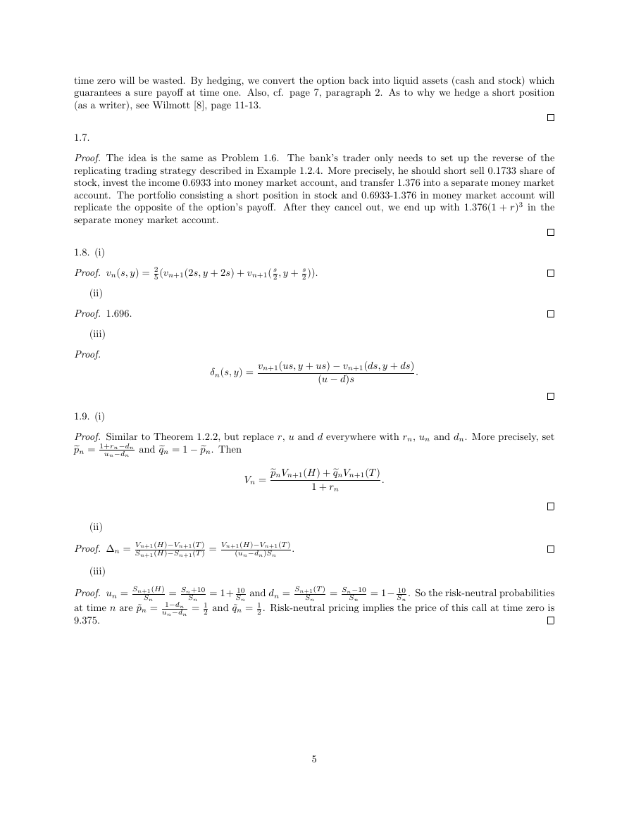
1.8. (i)
Proof. vn(s, y) = 2
5(vn+1(2s, y + 2s) + vn+1( s
2 , y + s
2)).
(ii)
Proof. 1.696.
(iii)
Proof.
δn(s, y) = vn+1(us, y + us) − vn+1(ds, y + ds)
(u − d)s
.
1.9. (i)
pn = 1+rn−dn
un−dn
and qn = 1 −pn. Then
Proof. Similar to Theorem 1.2.2, but replace r, u and d everywhere with rn, un and dn. More precisely, set
Vn = pnVn+1(H) +qnVn+1(T )
1 + rn
.
(ii)
Proof. ∆n = Vn+1(H)−Vn+1(T )
Sn+1(H)−Sn+1(T ) = Vn+1(H)−Vn+1(T )
(un−dn)Sn
.
(iii)
Proof. un = Sn+1(H)
at time n are ˜pn = 1−dn
un−dn
9.375.
= Sn+10
Sn
= 1
Sn
= 1+ 10
Sn
2 and ˜qn = 1
and dn = Sn+1(T )
. So the risk-neutral probabilities
2. Risk-neutral pricing implies the price of this call at time zero is
Sn
Sn
Sn
= Sn−10
= 1− 10
5
�
1.2 Probability Theory on Coin Toss Space
2.1. (i)
Proof. P (Ac) + P (A) =
ω∈A1∪A2 P (ω) =
ω∈Ac P (ω) +
ω∈A1 P (ω) +
(ii)
ω∈A P (ω) =
ω∈Ω P (ω) = 1.
Proof. By induction, it suffices to work on the case N = 2. When A1 and A2 are disjoint, P (A1 ∪ A2) =
ω∈A2 P (ω) = P (A1) + P (A2). When A1 and A2 are arbitrary, using
the result when they are disjoint, we have P (A1 ∪ A2) = P ((A1 − A2) ∪ A2) = P (A1 − A2) + P (A2) ≤
P (A1) + P (A2).
(ii)
2.2. (i)
8, P (S3 = 8) = 3p2q = 3
Proof. P (S3 = 32) =p3 = 1
Proof. E[S1] = 8P (S1 = 8) + 2P (S1 = 2) = 8p + 2q = 5, E[S2] = 16p2 + 4 · 2pq + 1 ·q2 = 6.25, and
E[S3] = 32 · 1
8 = 7.8125. So the average rates of growth of the stock price under P
are, respectively: r0 = 5
8 + 8 · 3
8, and P (S3 = 0.5) =q3 = 1
5 − 1 = 0.25 andr2 = 7.8125
8, P (S3 = 2) = 3pq2 = 3
4 − 1 = 0.25,r1 = 6.25
8 + 2 · 3
6.25 − 1 = 0.25.
8 + 0.5 · 1
8.
(iii)
Proof. P (S3 = 32) = ( 2
9, and P (S3 = 0.5) = 1
27.
Accordingly, E[S1] = 6, E[S2] = 9 and E[S3] = 13.5. So the average rates of growth of the stock price
3)3 = 8
9 = 2
27, P (S3 = 8) = 3 · ( 2
4 − 1 = 0.5, r1 = 9
3 = 4
9, P (S3 = 2) = 2 · 1
3)2 · 1
6 − 1 = 0.5, and r2 = 13.5
under P are, respectively: r0 = 6
9 − 1 = 0.5.
2.3.
Proof. Apply conditional Jensen’s inequality.
2.4. (i)
Proof. En[Mn+1] = Mn + En[Xn+1] = Mn + E[Xn+1] = Mn.
(ii)
Proof. En[ Sn+1
Sn
] = En[eσXn+1
2
eσ+e−σ ] =
2
eσ+e−σ E[eσXn+1] = 1.
2.5. (i)
Proof. 2In = 2n−1
n −n−1
j=0 Mj(Mj+1 − Mj) = 2n−1
n −n−1
j+1 −n−1
j = M 2
j=0 M 2
j=0 M 2
M 2
j=0 MjMj+1 −n−1
j=0 (Mj+1 − Mj)2 = M 2
j −n−1
j=1 M 2
n −n−1
j=0 X 2
j = 2n−1
j=1 M 2
j+1 = M 2
n − n.
j=0 MjMj+1 +
(ii)
Proof. En[f(In+1)] = En[f(In + Mn(Mn+1− Mn))] = En[f(In + MnXn+1)] = 1
g(In), where g(x) = 1
2x + n) + f(x − √
2In + n = |Mn|.
2x + n)], since
√
√
2[f(x +
2[f(In + Mn)+ f(In− Mn)] =
2.6.
Proof. En[In+1 − In] = En[∆n(Mn+1 − Mn)] = ∆nEn[Mn+1 − Mn] = 0.
2.7.
6
�
Proof. We denote by Xn the result of n-th coin toss, where Head is represented by X = 1 and Tail is
represented by X = −1. We also suppose P (X = 1) = P (X = −1) = 1
2. Define S1 = X1 and Sn+1 =
Sn +bn(X1,··· , Xn)Xn+1, where bn(·) is a bounded function on {−1, 1}n, to be determined later on. Clearly
(Sn)n≥1 is an adapted stochastic process, and we can show it is a martingale. Indeed, En[Sn+1 − Sn] =
bn(X1,··· , Xn)En[Xn+1] = 0.
2[f(Sn + bn(X1,··· , Xn)) + f(Sn − bn(X1,··· , Xn))]. Then
intuitively, En[f(Sn+1] cannot be solely dependent upon Sn when bn’s are properly chosen. Therefore in
general, (Sn)n≥1 cannot be a Markov process.
Remark 1. If Xn is regarded as the gain/loss of n-th bet in a gambling game, then Sn would be the wealth
at time n. bn is therefore the wager for the (n+1)-th bet and is devised according to past gambling results.
For any arbitrary function f, En[f(Sn+1)] = 1
2.8. (i)
Proof. Note Mn = En[MN ] and M
n = En[M
N ].
(ii)
Proof. In the proof of Theorem 1.2.2, we proved by induction that Xn = Vn where Xn is defined by (1.2.14)
of Chapter 1. In other words, the sequence (Vn)0≤n≤N can be realized as the value process of a portfolio,
which consists of stock and money market accounts. Since ( Xn
2.4.5), ( Vn
(1+r)n )0≤n≤N is a martingale under P (Theorem
(1+r)n )0≤n≤N is a martingale under P .
VN
(1+r)N
(iii)
Proof.
(iv)
V
(1+r)n = En
n
, so V
0, V
1+r , ··· ,
1
(1+r)N is a martingale under P .
VN
V
N−1
(1+r)N−1 ,
Proof. Combine (ii) and (iii), then use (i).
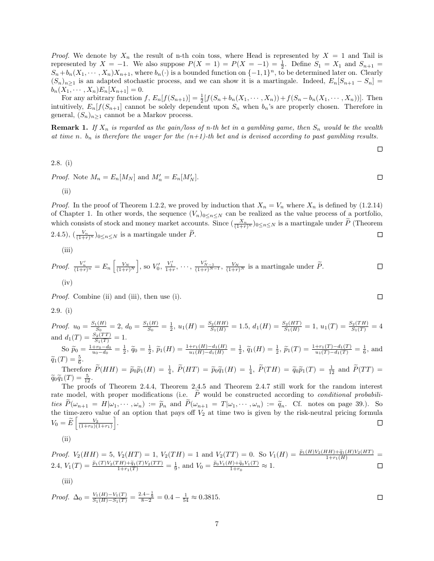
2.9. (i)
S0
Proof. u0 = S1(H)
and d1(T ) = S2(T T )
S1(T ) = 1.
= 1
u0−d0
= 2, d0 = S1(H)
S0
= 1
2, u1(H) = S2(HH)
S1(H) = 1.5, d1(H) = S2(HT )
S1(H) = 1, u1(T ) = S2(T H)
S1(T ) = 4
6.
12.
u1(T )−d1(T ) = 1
2, q0 = 1
2, p1(H) = 1+r1(H)−d1(H)
u1(H)−d1(H) = 1
2, p1(T ) = 1+r1(T )−d1(T )
4, P (HT ) = p0q1(H) = 1
The proofs of Theorem 2.4.4, Theorem 2.4.5 and Theorem 2.4.7 still work for the random interest
2, q1(H) = 1
4, P (T H) = q0p1(T ) = 1
So p0 = 1+r0−d0
q1(T ) = 5
Therefore P (HH) = p0p1(H) = 1
12 and P (T T ) =
q0q1(T ) = 5
rate model, with proper modifications (i.e. P would be constructed according to conditional probabili-
ties P (ωn+1 = H|ω1,··· , ωn) := pn and P (ωn+1 = T|ω1,··· , ωn) := qn. Cf. notes on page 39.). So
V0 = E
Proof. V2(HH) = 5, V2(HT ) = 1, V2(T H) = 1 and V2(T T ) = 0. So V1(H) = p1(H)V2(HH)+q1(H)V2(HT )
2.4, V1(T ) = p1(T )V2(T H)+q1(T )V2(T T )
the time-zero value of an option that pays off V2 at time two is given by the risk-neutral pricing formula
9, and V0 = p0V1(H)+q0V1(T )
6, and
(1+r0)(1+r1)
≈ 1.
1+r1(H)
= 1
(ii)
=
V2
.
1+r1(T )
1+r0
(iii)
Proof. ∆0 = V1(H)−V1(T )
S1(H)−S1(T ) = 2.4− 1
8−2 = 0.4 − 1
54 ≈ 0.3815.
9
7
�




 2023年江西萍乡中考道德与法治真题及答案.doc
 2012年重庆南川中考生物真题及答案.doc
 2013年江西师范大学地理学综合及文艺理论基础考研真题.doc
 2020年四川甘孜小升初语文真题及答案I卷.doc
 2020年注册岩土工程师专业基础考试真题及答案.doc
 2023-2024学年福建省厦门市九年级上学期数学月考试题及答案.doc
 2021-2022学年辽宁省沈阳市大东区九年级上学期语文期末试题及答案.doc
 2022-2023学年北京东城区初三第一学期物理期末试卷及答案.doc
 2018上半年江西教师资格初中地理学科知识与教学能力真题及答案.doc
 2012年河北国家公务员申论考试真题及答案-省级.doc
 2020-2021学年江苏省扬州市江都区邵樊片九年级上学期数学第一次质量检测试题及答案.doc
 2022下半年黑龙江教师资格证中学综合素质真题及答案.doc