IEEE TRANSACTIONS ON PATTERN ANALYSIS AND MACHINE INTELLIGENCE, VOL. 34, NO. 4, APRIL 2012
743
Pedestrian Detection:
An Evaluation of the State of the Art
Piotr Dolla´ r, Christian Wojek, Bernt Schiele, and Pietro Perona
Abstract—Pedestrian detection is a key problem in computer vision, with several applications that have the potential to positively
impact quality of life. In recent years, the number of approaches to detecting pedestrians in monocular images has grown steadily.
However, multiple data sets and widely varying evaluation protocols are used, making direct comparisons difficult. To address these
shortcomings, we perform an extensive evaluation of the state of the art in a unified framework. We make three primary contributions:
1) We put together a large, well-annotated, and realistic monocular pedestrian detection data set and study the statistics of the size,
position, and occlusion patterns of pedestrians in urban scenes, 2) we propose a refined per-frame evaluation methodology that allows
us to carry out probing and informative comparisons, including measuring performance in relation to scale and occlusion, and 3) we
evaluate the performance of sixteen pretrained state-of-the-art detectors across six data sets. Our study allows us to assess the state
of the art and provides a framework for gauging future efforts. Our experiments show that despite significant progress, performance
still has much room for improvement. In particular, detection is disappointing at low resolutions and for partially occluded pedestrians.
Index Terms—Pedestrian detection, object detection, benchmark, evaluation, data set, Caltech Pedestrian data set.
Ç
1 INTRODUCTION
PEOPLE are among the most important components of a
machine’s environment, and endowing machines with
the ability to interact with people is one of the most
interesting and potentially useful challenges for modern
engineering. Detecting and tracking people is thus an
important area of research, and machine vision is bound
to play a key role. Applications include robotics, entertain-
ment, surveillance, care for the elderly and disabled, and
content-based indexing. Just in the US, nearly 5,000 of the
35,000 annual traffic crash fatalities involve pedestrians [1];
hence the considerable interest
in building automated
vision systems for detecting pedestrians [2].
While there is much ongoing research in machine
vision approaches for detecting pedestrians, varying
evaluation protocols and use of different data sets makes
direct comparisons difficult. Basic questions such as “Do
current detectors work well?” “What
is the best ap-
proach?” “What are the main failure modes?” and “What
are the most productive research directions?” are not
easily answered.
Our study aims to address these questions. We focus on
methods for detecting pedestrians in individual monocular
images; for an overview of how detectors are incorporated
into full systems we refer readers to [2]. Our approach is
three-pronged: We collect, annotate, and study a large data
. P. Dolla´r and P. Perona are with the Department of Electrical Engineering,
California Institute of Technology, MC 136-93, 1200 E. California Blvd.,
Pasadena, CA 91125. E-mail: {pdollar, perona}@caltech.edu.
. C. Wojek and B. Schiele are with the Max Planck Institute for Informatics,
Campus E1 4, Saarbru¨cken 66123, Germany.
E-mail: {cwojek, schiele}@mpi-inf.mpg.de.
Manuscript received 2 Nov. 2010; revised 17 June 2011; accepted 3 July 2011;
published online 28 July 2011.
Recommended for acceptance by G. Mori.
For information on obtaining reprints of this article, please send e-mail to:
tpami@computer.org, and reference IEEECS Log Number
TPAMI-2010-11-0837.
Digital Object Identifier no. 10.1109/TPAMI.2011.155.
set of pedestrian images collected from a vehicle navigating in
urban traffic; we develop informative evaluation methodol-
ogies and point out pitfalls in previous experimental
procedures; finally, we compare the performance of 16 pre-
trained pedestrian detectors on six publicly available data
sets, including our own. Our study allows us to assess the
state of the art and suggests directions for future research.
All results of this study, and the data and tools for
reproducing them, are posted on the project website: www.
vision.caltech.edu/Image_Datasets/CaltechPedestrians/.
1.1 Contributions
Data set. In earlier work [3], we introduced the Caltech
Pedestrian Data Set, which includes 350,000 pedestrian
bounding boxes (BB) labeled in 250,000 frames and remains
the largest such data set to date. Occlusions and temporal
correspondences are also annotated. Using the extensive
ground truth, we analyze the statistics of pedestrian scale,
occlusion, and location and help establish conditions under
which detection systems must operate.
Evaluation methodology. We aim to quantify and rank
detector performance in a realistic and unbiased manner. To
this effect, we explore a number of choices in the evaluation
protocol and their effect on reported performance. Overall,
the methodology has changed substantially since [3],
resulting in a more accurate and informative benchmark.
Evaluation. We evaluate 16 representative state-of-the-
art pedestrian detectors (previously we evaluated seven
[3]). Our goal was to choose diverse detectors that were
most promising in terms of originally reported perfor-
mance. We avoid retraining or modifying the detectors to
ensure each method was optimized by its authors. In
addition to overall performance, we explore detection rates
under varying levels of scale and occlusion and on clearly
visible pedestrians. Moreover, we measure localization
accuracy and analyze runtime.
To increase the scope of our analysis, we also benchmark
the 16 detectors using a unified evaluation framework on
0162-8828/12/$31.00 ß 2012 IEEE
Published by the IEEE Computer Society
�
744
IEEE TRANSACTIONS ON PATTERN ANALYSIS AND MACHINE INTELLIGENCE, VOL. 34, NO. 4, APRIL 2012
Fig. 2. Overview of the Caltech Pedestrian Data Set. (a) Camera setup.
(b) Summary of data set statistics (1k ¼ 103). The data set is large,
realistic, and well annotated, allowing us to study statistics of the size,
position, and occlusion of pedestrians in urban scenes and also to
accurately evaluate the state or the art in pedestrian detection.
Middlebury Stereo Data Set [11], and the Caltech 101 [12],
Caltech 256 [13], and PASCAL [14] object recognition data
sets all improved performance evaluation, added challenge,
and helped drive innovation in their respective fields. Much
in the same way, our goal
in introducing the Caltech
Pedestrian Data Set is to provide a better benchmark and to
help identify conditions under which current detectors fail
and thus focus research effort on these difficult cases.
2.1 Data Collection and Ground Truthing
We collected approximately 10 hours of 30 Hz video
(� 106 frames) taken from a vehicle driving through regular
traffic in an urban environment (camera setup shown in
Fig. 2a). The CCD video resolution is 640 � 480, and, not
unexpectedly, the overall image quality is lower than that of
still
images of comparable resolution. There are minor
variations in the camera position due to repeated mount-
ings of the camera. The driver was independent from the
authors of this study and had instructions to drive normally
through neighborhoods in the greater Los Angeles metro-
politan area chosen for their relatively high concentration of
pedestrians,
including LAX, Santa Monica, Hollywood,
Pasadena, and Little Tokyo. In order to remove effects of the
vehicle pitching and thus simplify annotation, the video
was stabilized using the inverse compositional algorithm
for image alignment by Baker and Matthews [15].
After video stabilization, 250,000 frames (in 137 approxi-
mately minute long segments extracted from the 10 hours of
video) were annotated for a total of 350,000 bounding boxes
around 2,300 unique pedestrians. To make such a large
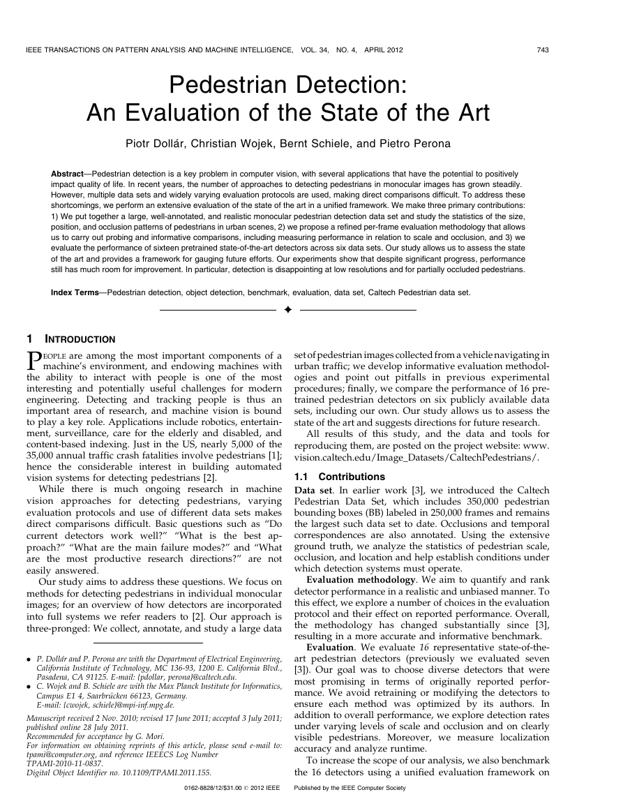
scale labeling effort feasible we created a user-friendly
labeling tool, shown in Fig. 3. Its most salient aspect is an
interactive procedure where the annotator labels a sparse
set of
frames and the system automatically predicts
pedestrian positions in intermediate frames. Specifically,
after an annotator labels a bounding box around the same
pedestrian in at least two frames, BBs in intermediate
frames are interpolated using cubic interpolation (applied
independently to each coordinate of the BBs). Thereafter,
every time an annotator alters a BB, BBs in all the unlabeled
frames are reinterpolated. The annotator continues until
satisfied with the result. We experimented with more
sophisticated interpolation schemes, including relying on
tracking; however, cubic interpolation proved best. Label-
ing the �2:3 hours of video, including verification, took
�400 hours total (spread across multiple annotators).
Fig. 1. Example images (cropped) and annotations from six pedestrian
detection data sets. We perform an extensive evaluation of pedestrian
detection, benchmarking 16 detectors on each of these six data sets. By
using multiple data sets and a unified evaluation framework we can draw
broad conclusion about the state of the art and suggest future research
directions.
six additional pedestrian detection data sets, including the
ETH [4], TUD-Brussels [5], Daimler [6], and INRIA [7] data
sets and two variants of the Caltech data set (see Fig. 1). By
evaluating across multiple data sets, we can rank detector
performance and analyze the statistical significance of the
results and, more generally, draw conclusions both about
the detectors and the data sets themselves.
Two groups have recently published surveys which are
complementary to our own. Geronimo et al. [2] performed a
comprehensive survey of pedestrian detection for advanced
driver assistance systems, with a clear focus on full systems.
Enzweiler and Gavrila [6] published the Daimler detection
data set and an accompanying evaluation of three detectors,
performing additional experiments integrating the detec-
tors into full systems. We instead focus on a more thorough
and detailed evaluation of state-of-the-art detectors.
This paper is organized as follows: We introduce the
Caltech Pedestrian Data Set and analyze its statistics in
Section 2; a comparison of existing data sets is given in
Section 2.4. In Section 3, we discuss evaluation methodology
in detail. A survey of pedestrian detectors is given in
Section 4.1 and in Section 4.2 we discuss the 16 representative
state-of-the-art detectors used in our evaluation. In Section 5,
we report the results of the performance evaluation, both
under varying conditions using the Caltech data set and on
six additional data sets. We conclude with a discussion of the
state of the art in pedestrian detection in Section 6.
2 THE CALTECH PEDESTRIAN DATA SET
Challenging data sets are catalysts for progress in computer
vision. The Barron et al. [8] and Middlebury [9] optical flow
data sets, the Berkeley Segmentation Data Set [10], the
�
DOLL�AR ET AL.: PEDESTRIAN DETECTION: AN EVALUATION OF THE STATE OF THE ART
745
Fig. 3. The annotation tool allows annotators to efficiently navigate and
annotate a video in a minimum amount of time. Its most salient aspect is
an interactive procedure where the annotator labels only a sparse set of
frames and the system automatically predicts pedestrian positions in
intermediate frames. The annotation tool
is available on the project
website.
For every frame in which a given pedestrian is visible,
annotators mark a BB that indicates the full extent of the
entire pedestrian (BB-full); for occluded pedestrians this
involves estimating the location of hidden parts. In addition
a second BB is used to delineate the visible region (BB-vis),
see Fig. 5a. During an occlusion event, the estimated full BB
stays relatively constant while the visible BB may change
rapidly. For comparison, in the PASCAL labeling scheme
[14] only the visible BB is labeled and occluded objects are
marked as “truncated.”
Each sequence of BBs belonging to a single object was
assigned one of three labels. Individual pedestrians were
labeled “Person” (� 1;900 instances). Large groups for
which it would have been tedious or impossible to label
individuals were delineated using a single BB and labeled
as “People” (� 300). In addition, the label “Person?” was
assigned when clear identification of a pedestrian was
ambiguous or easily mistaken (� 110).
2.2 Data Set Statistics
A summary of the data set is given in Fig. 2b. About
50 percent of
the frames have no pedestrians, while
30 percent have two or more, and pedestrians are visible
for 5 s on average. Below, we analyze the distribution of
pedestrian scale, occlusion, and location. This serves to
establish the requirements of a real world system and to
help identify constraints that can be used to improve
automatic pedestrian detection systems.
2.2.1 Scale Statistics
We group pedestrians by their image size (height in pixels)
into three scales: near (80 or more pixels), medium
(between 30-80 pixels), and far (30 pixels or less). This
division into three scales is motivated by the distribution of
sizes in the data set, human performance, and automotive
system requirements.
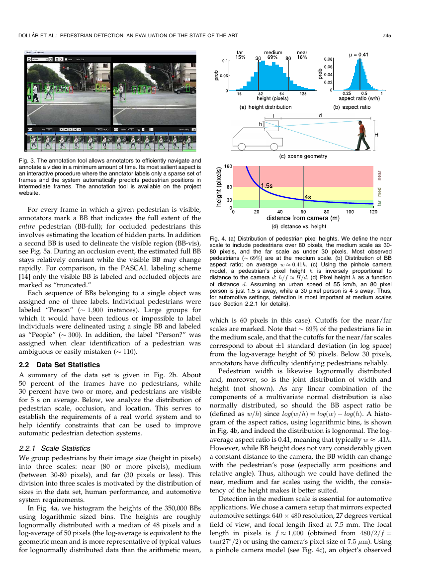
In Fig. 4a, we histogram the heights of the 350,000 BBs
using logarithmic sized bins. The heights are roughly
lognormally distributed with a median of 48 pixels and a
log-average of 50 pixels (the log-average is equivalent to the
geometric mean and is more representative of typical values
for lognormally distributed data than the arithmetic mean,
Fig. 4. (a) Distribution of pedestrian pixel heights. We define the near
scale to include pedestrians over 80 pixels, the medium scale as 30-
80 pixels, and the far scale as under 30 pixels. Most observed
pedestrians (� 69%) are at the medium scale. (b) Distribution of BB
aspect ratio; on average w � 0:41h. (c) Using the pinhole camera
model, a pedestrian’s pixel height h is inversely proportional
to
distance to the camera d: h=f � H=d. (d) Pixel height h as a function
of distance d. Assuming an urban speed of 55 km/h, an 80 pixel
person is just 1.5 s away, while a 30 pixel person is 4 s away. Thus,
for automotive settings, detection is most important at medium scales
(see Section 2.2.1 for details).
which is 60 pixels in this case). Cutoffs for the near/far
scales are marked. Note that � 69% of the pedestrians lie in
the medium scale, and that the cutoffs for the near/far scales
correspond to about �1 standard deviation (in log space)
from the log-average height of 50 pixels. Below 30 pixels,
annotators have difficulty identifying pedestrians reliably.
Pedestrian width is likewise lognormally distributed
and, moreover, so is the joint distribution of width and
height (not shown). As any linear combination of the
components of a multivariate normal distribution is also
normally distributed, so should the BB aspect ratio be
(defined as w=h) since logðw=hÞ ¼ logðwÞ � logðhÞ. A histo-
gram of the aspect ratios, using logarithmic bins, is shown
in Fig. 4b, and indeed the distribution is lognormal. The log-
average aspect ratio is 0.41, meaning that typically w � :41h.
However, while BB height does not vary considerably given
a constant distance to the camera, the BB width can change
with the pedestrian’s pose (especially arm positions and
relative angle). Thus, although we could have defined the
near, medium and far scales using the width, the consis-
tency of the height makes it better suited.
Detection in the medium scale is essential for automotive
applications. We chose a camera setup that mirrors expected
automotive settings: 640 � 480 resolution, 27 degrees vertical
field of view, and focal length fixed at 7.5 mm. The focal
length in pixels is f � 1;000 (obtained from 480=2=f ¼
tanð27�=2Þ or using the camera’s pixel size of 7:5 �m). Using
a pinhole camera model (see Fig. 4c), an object’s observed
�
746
IEEE TRANSACTIONS ON PATTERN ANALYSIS AND MACHINE INTELLIGENCE, VOL. 34, NO. 4, APRIL 2012
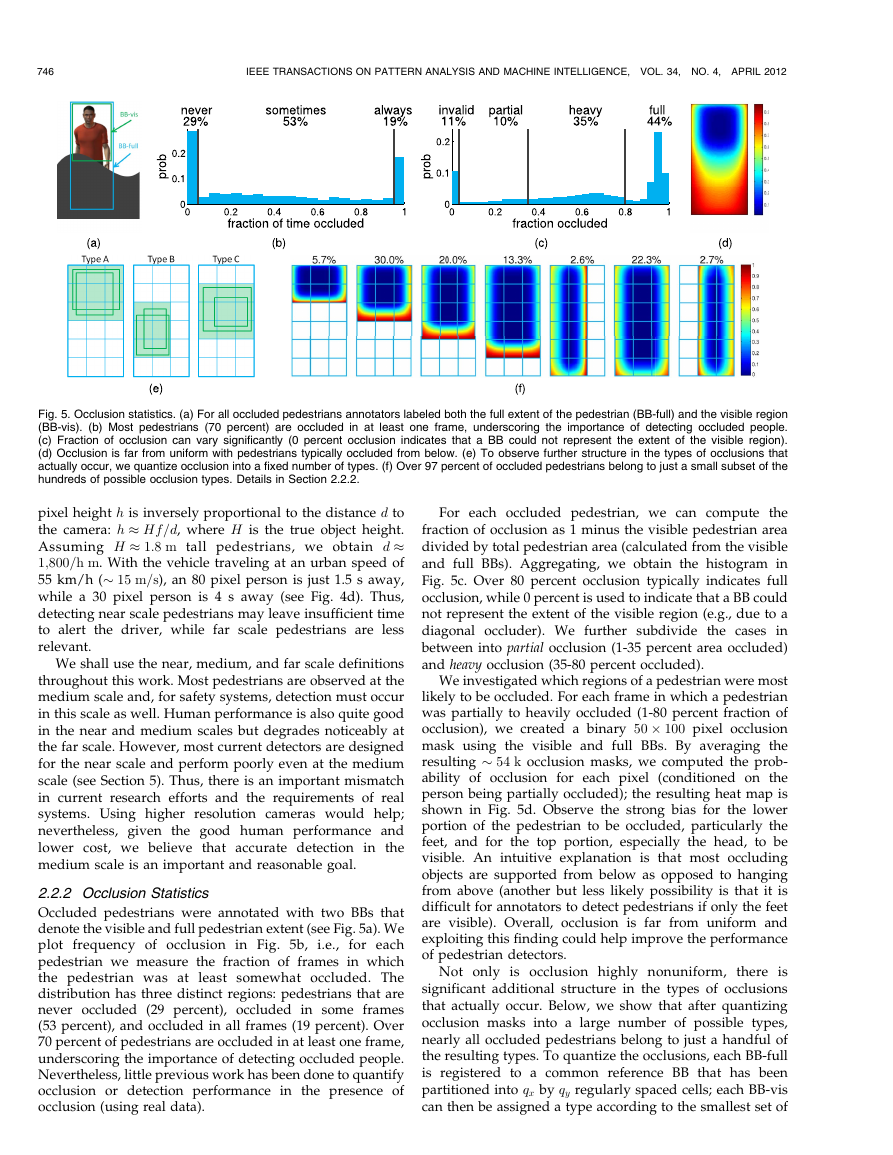
Fig. 5. Occlusion statistics. (a) For all occluded pedestrians annotators labeled both the full extent of the pedestrian (BB-full) and the visible region
(BB-vis). (b) Most pedestrians (70 percent) are occluded in at least one frame, underscoring the importance of detecting occluded people.
(c) Fraction of occlusion can vary significantly (0 percent occlusion indicates that a BB could not represent the extent of the visible region).
(d) Occlusion is far from uniform with pedestrians typically occluded from below. (e) To observe further structure in the types of occlusions that
actually occur, we quantize occlusion into a fixed number of types. (f) Over 97 percent of occluded pedestrians belong to just a small subset of the
hundreds of possible occlusion types. Details in Section 2.2.2.
pixel height h is inversely proportional to the distance d to
the camera: h � Hf=d, where H is the true object height.
Assuming H � 1:8 m tall pedestrians, we obtain d �
1;800=h m. With the vehicle traveling at an urban speed of
55 km/h (� 15 m=s), an 80 pixel person is just 1.5 s away,
while a 30 pixel person is 4 s away (see Fig. 4d). Thus,
detecting near scale pedestrians may leave insufficient time
to alert the driver, while far scale pedestrians are less
relevant.
We shall use the near, medium, and far scale definitions
throughout this work. Most pedestrians are observed at the
medium scale and, for safety systems, detection must occur
in this scale as well. Human performance is also quite good
in the near and medium scales but degrades noticeably at
the far scale. However, most current detectors are designed
for the near scale and perform poorly even at the medium
scale (see Section 5). Thus, there is an important mismatch
in current research efforts and the requirements of real
systems. Using higher resolution cameras would help;
nevertheless, given the good human performance and
lower cost, we believe that accurate detection in the
medium scale is an important and reasonable goal.
i.e.,
frequency of occlusion in Fig. 5b,
2.2.2 Occlusion Statistics
Occluded pedestrians were annotated with two BBs that
denote the visible and full pedestrian extent (see Fig. 5a). We
plot
for each
pedestrian we measure the fraction of frames in which
the pedestrian was at
least somewhat occluded. The
distribution has three distinct regions: pedestrians that are
never occluded (29 percent), occluded in some frames
(53 percent), and occluded in all frames (19 percent). Over
70 percent of pedestrians are occluded in at least one frame,
underscoring the importance of detecting occluded people.
Nevertheless, little previous work has been done to quantify
occlusion or detection performance in the presence of
occlusion (using real data).
For each occluded pedestrian, we can compute the
fraction of occlusion as 1 minus the visible pedestrian area
divided by total pedestrian area (calculated from the visible
and full BBs). Aggregating, we obtain the histogram in
Fig. 5c. Over 80 percent occlusion typically indicates full
occlusion, while 0 percent is used to indicate that a BB could
not represent the extent of the visible region (e.g., due to a
diagonal occluder). We further subdivide the cases in
between into partial occlusion (1-35 percent area occluded)
and heavy occlusion (35-80 percent occluded).
We investigated which regions of a pedestrian were most
likely to be occluded. For each frame in which a pedestrian
was partially to heavily occluded (1-80 percent fraction of
occlusion), we created a binary 50 � 100 pixel occlusion
mask using the visible and full BBs. By averaging the
resulting � 54 k occlusion masks, we computed the prob-
ability of occlusion for each pixel (conditioned on the
person being partially occluded); the resulting heat map is
shown in Fig. 5d. Observe the strong bias for the lower
portion of the pedestrian to be occluded, particularly the
feet, and for the top portion, especially the head, to be
visible. An intuitive explanation is that most occluding
objects are supported from below as opposed to hanging
from above (another but less likely possibility is that it is
difficult for annotators to detect pedestrians if only the feet
are visible). Overall, occlusion is far from uniform and
exploiting this finding could help improve the performance
of pedestrian detectors.
Not only is occlusion highly nonuniform,
there is
significant additional structure in the types of occlusions
that actually occur. Below, we show that after quantizing
occlusion masks into a large number of possible types,
nearly all occluded pedestrians belong to just a handful of
the resulting types. To quantize the occlusions, each BB-full
is registered to a common reference BB that has been
partitioned into qx by qy regularly spaced cells; each BB-vis
can then be assigned a type according to the smallest set of
�
DOLL�AR ET AL.: PEDESTRIAN DETECTION: AN EVALUATION OF THE STATE OF THE ART
747
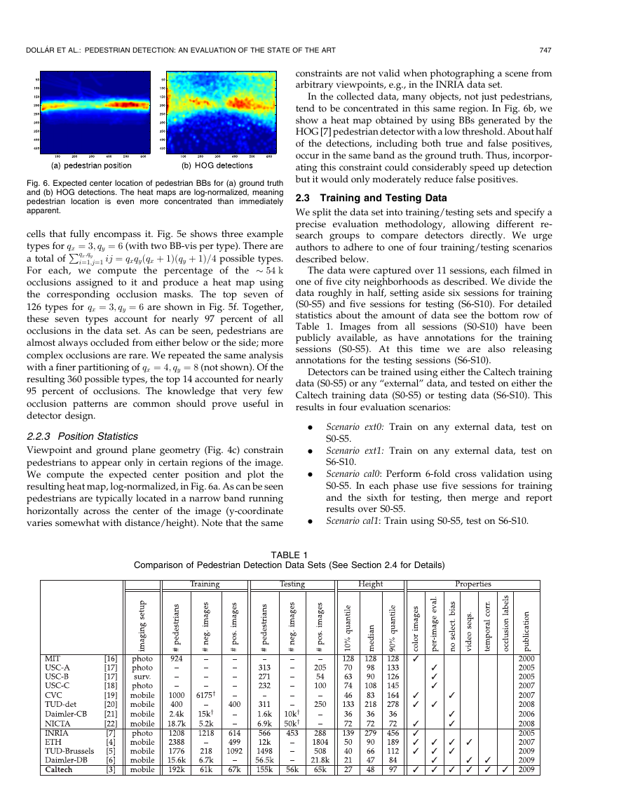
constraints are not valid when photographing a scene from
arbitrary viewpoints, e.g., in the INRIA data set.
In the collected data, many objects, not just pedestrians,
tend to be concentrated in this same region. In Fig. 6b, we
show a heat map obtained by using BBs generated by the
HOG [7] pedestrian detector with a low threshold. About half
of the detections, including both true and false positives,
occur in the same band as the ground truth. Thus, incorpor-
ating this constraint could considerably speed up detection
but it would only moderately reduce false positives.
2.3 Training and Testing Data
We split the data set into training/testing sets and specify a
precise evaluation methodology, allowing different re-
search groups to compare detectors directly. We urge
authors to adhere to one of four training/testing scenarios
described below.
The data were captured over 11 sessions, each filmed in
one of five city neighborhoods as described. We divide the
data roughly in half, setting aside six sessions for training
(S0-S5) and five sessions for testing (S6-S10). For detailed
statistics about the amount of data see the bottom row of
Table 1.
Images from all sessions (S0-S10) have been
publicly available, as have annotations for the training
sessions (S0-S5). At
this time we are also releasing
annotations for the testing sessions (S6-S10).
Detectors can be trained using either the Caltech training
data (S0-S5) or any “external” data, and tested on either the
Caltech training data (S0-S5) or testing data (S6-S10). This
results in four evaluation scenarios:
.
.
.
.
Scenario ext0: Train on any external data, test on
S0-S5.
Scenario ext1: Train on any external data, test on
S6-S10.
Scenario cal0: Perform 6-fold cross validation using
S0-S5. In each phase use five sessions for training
and the sixth for testing, then merge and report
results over S0-S5.
Scenario cal1: Train using S0-S5, test on S6-S10.
Fig. 6. Expected center location of pedestrian BBs for (a) ground truth
and (b) HOG detections. The heat maps are log-normalized, meaning
pedestrian location is even more concentrated than immediately
apparent.
qx;qy
P
cells that fully encompass it. Fig. 5e shows three example
types for qx ¼ 3; qy ¼ 6 (with two BB-vis per type). There are
i¼1;j¼1 ij ¼ qxqyðqx þ 1Þðqy þ 1Þ=4 possible types.
a total of
the � 54 k
For each, we compute the percentage of
occlusions assigned to it and produce a heat map using
the corresponding occlusion masks. The top seven of
126 types for qx ¼ 3; qy ¼ 6 are shown in Fig. 5f. Together,
these seven types account for nearly 97 percent of all
occlusions in the data set. As can be seen, pedestrians are
almost always occluded from either below or the side; more
complex occlusions are rare. We repeated the same analysis
with a finer partitioning of qx ¼ 4; qy ¼ 8 (not shown). Of the
resulting 360 possible types, the top 14 accounted for nearly
95 percent of occlusions. The knowledge that very few
occlusion patterns are common should prove useful
in
detector design.
2.2.3 Position Statistics
Viewpoint and ground plane geometry (Fig. 4c) constrain
pedestrians to appear only in certain regions of the image.
We compute the expected center position and plot the
resulting heat map, log-normalized, in Fig. 6a. As can be seen
pedestrians are typically located in a narrow band running
horizontally across the center of the image (y-coordinate
varies somewhat with distance/height). Note that the same
Comparison of Pedestrian Detection Data Sets (See Section 2.4 for Details)
TABLE 1
�
748
IEEE TRANSACTIONS ON PATTERN ANALYSIS AND MACHINE INTELLIGENCE, VOL. 34, NO. 4, APRIL 2012
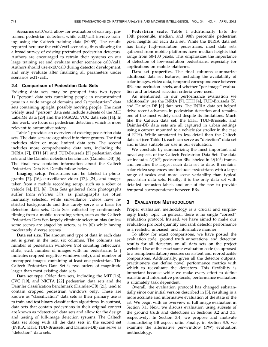
Scenarios ext0/ext1 allow for evaluation of existing, pre-
trained pedestrian detectors, while cal0/cal1 involve train-
ing using the Caltech training data (S0-S5). The results
reported here use the ext0/ext1 scenarios, thus allowing for
a broad survey of existing pretrained pedestrian detectors.
Authors are encouraged to retrain their systems on our
large training set and evaluate under scenarios cal0/cal1.
Authors should use ext0/cal0 during detector development,
and only evaluate after finalizing all parameters under
scenarios ext1/cal1.
2.4 Comparison of Pedestrian Data Sets
Existing data sets may be grouped into two types:
1) “person” data sets containing people in unconstrained
pose in a wide range of domains and 2) “pedestrian” data
sets containing upright, possibly moving people. The most
widely used “person” data sets include subsets of the MIT
LabelMe data [23] and the PASCAL VOC data sets [14]. In
this work, we focus on pedestrian detection, which is more
relevant to automotive safety.
Table 1 provides an overview of existing pedestrian data
sets. The data sets are organized into three groups. The first
includes older or more limited data sets. The second
includes more comprehensive data sets,
including the
INRIA [7], ETH [4], and TUD-Brussels [5] pedestrian data
sets and the Daimler detection benchmark (Daimler-DB) [6].
The final row contains information about
the Caltech
Pedestrian Data Set. Details follow below.
Imaging setup. Pedestrians can be labeled in photo-
graphs [7], [16], surveillance video [17], [24], and images
taken from a mobile recording setup, such as a robot or
vehicle [4], [5], [6]. Data Sets gathered from photographs
suffer from selection bias, as photographs are often
manually selected, while surveillance videos have re-
stricted backgrounds and thus rarely serve as a basis for
detection data sets. Data Sets collected by continuously
filming from a mobile recording setup, such as the Caltech
Pedestrian Data Set, largely eliminate selection bias (unless
some scenes are staged by actors, as in [6]) while having
moderately diverse scenes.
Data set size. The amount and type of data in each data
set is given in the next six columns. The columns are:
number of pedestrian windows (not counting reflections,
shifts, etc.), number of images with no pedestrians (a y
indicates cropped negative windows only), and number of
uncropped images containing at least one pedestrian. The
Caltech Pedestrian Data Set is two orders of magnitude
larger than most existing data sets.
Data set type. Older data sets, including the MIT [16],
CVC [19], and NICTA [22] pedestrian data sets and the
Daimler classification benchmark (Daimler-CB) [21], tend to
contain cropped pedestrian windows only. These are
known as “classification” data sets as their primary use is
to train and test binary classification algorithms. In contrast,
data sets that contain pedestrians in their original context
are known as “detection” data sets and allow for the design
and testing of full-image detection systems. The Caltech
data set along with all the data sets in the second set
(INRIA, ETH, TUD-Brussels, and Daimler-DB) can serve as
“detection” data sets.
Pedestrian scale. Table 1 additionally lists
the
10th percentile, median, and 90th percentile pedestrian
pixel heights for each data set. While the INRIA data set
has fairly high-resolution pedestrians, most data sets
gathered from mobile platforms have median heights that
range from 50-100 pixels. This emphasizes the importance
of detection of low-resolution pedestrians, especially for
applications on mobile platforms.
Data set properties. The final columns summarize
additional data set features, including the availability of
color images, video data, temporal correspondence between
BBs and occlusion labels, and whether “per-image” evalua-
tion and unbiased selection criteria were used.
As mentioned,
in our performance evaluation we
additionally use the INRIA [7], ETH [4], TUD-Brussels [5],
and Daimler-DB [6] data sets. The INRIA data set helped
drive recent advances in pedestrian detection and remains
one of the most widely used despite its limitations. Much
like the Caltech data set, the ETH, TUD-Brussels, and
Daimler-DB data sets are all captured in urban settings
using a camera mounted to a vehicle (or stroller in the case
of ETH). While annotated in less detail than the Caltech
data set (see Table 1), each can serve as “detection” data set
and is thus suitable for use in our evaluation.
We conclude by summarizing the most important and
novel aspects of the Caltech Pedestrian Data Set. The data
set includes Oð105Þ pedestrian BBs labeled in Oð105Þ frames
and remains the largest such data set to date. It contains
color video sequences and includes pedestrians with a large
range of scales and more scene variability than typical
pedestrian data sets. Finally, it is the only data set with
detailed occlusion labels and one of the few to provide
temporal correspondence between BBs.
3 EVALUATION METHODOLOGY
Proper evaluation methodology is a crucial and surpris-
ingly tricky topic. In general, there is no single “correct”
evaluation protocol. Instead, we have aimed to make our
evaluation protocol quantify and rank detector performance
in a realistic, unbiased, and informative manner.
To allow for exact comparisons, we have posted the
evaluation code, ground truth annotations, and detection
results for all detectors on all data sets on the project
website. Use of the exact same evaluation code (as opposed
to a reimplementation) ensures consistent and reproducible
comparisons. Additionally, given all the detector outputs,
practitioners can define novel performance metrics with
which to reevaluate the detectors. This flexibility is
important because while we make every effort to define
realistic and informative protocols, performance evaluation
is ultimately task dependent.
Overall, the evaluation protocol has changed substan-
tially since our initial version described in [3], resulting in a
more accurate and informative evaluation of the state of the
art. We begin with an overview of full image evaluation in
Section 3.1. Next, we discuss evaluation using subsets of
the ground truth and detections in Sections 3.2 and 3.3,
respectively.
In Section 3.4, we propose and motivate
standardizing BB aspect ratio. Finally, in Section 3.5, we
examine the alternative per-window (PW) evaluation
methodology.
�
DOLL�AR ET AL.: PEDESTRIAN DETECTION: AN EVALUATION OF THE STATE OF THE ART
749
the log-average miss rate is similar to the performance at
10�1 FPPI but
in general gives a more stable and
informative assessment of performance. A similar perfor-
mance measure was used in [27].
We conclude by listing additional details. Some detec-
tors output BBs with padding around the pedestrian (e.g.,
HOG outputs 128 � 64 BBs around 96 pixel tall people),
such padding is cropped (see also Section 3.4). Methods
usually detect pedestrians at some minimum size; to coax
smaller detections, we upscale the input
images. For
ground truth, the full BB is always used for matching,
not the visible BB, even for partially occluded pedestrians.
Finally, all reported results on the Caltech data set are
computed using every 30th frame (starting with the
30th frame) due to the high-computational demands of
some of the detectors evaluated (see Fig. 15).
3.2 Filtering Ground Truth
Often we wish to exclude portions of a data set during
evaluation. This serves two purposes: 1) excluding ambig-
uous regions, e.g., crowds annotated as “People” where the
locations of individuals is unknown, and 2) evaluating
performance on various subsets of a data set, e.g., on
pedestrians in a given scale range. However, we cannot
simply discard a subset of ground truth labels as this would
cause overreporting of false positives.
Instead, to exclude portions of a data set, we introduce
the notion of ignore regions. Ground truth BBs selected to be
ignored, denoted using BBig, need not be matched;
however, matches are not considered mistakes either. For
example, to evaluate performance on unoccluded pedes-
trians, we set all occluded pedestrian BBs to ignore.
Evaluation is purposely lenient: Multiple detections can
match a single BBig; moreover, a detection may match any
subregion of a BBig. This is useful when the number or
location of pedestrians within a single BBig is unknown as
in the case of groups labeled as “People.”
In the proposed criterion, a BBdt can match any
subregion of a BBig. The subregion that maximizes area of
is BBdt \ BBig, and the resulting
overlap (1) with BBdt
maximum area of overlap is
ao ¼: areaðBBdt \ BBigÞ
areaðBBdtÞ
:
ð2Þ
Matching proceeds as before, except BBdt matched to BBig
do not count as true positives and unmatched BBig do not
count as false negatives. Matches to BBgt are preferred,
meaning a BBdt can only match a BBig if it does not match
any BBgt, and multiple matches to a single BBig are allowed.
As discussed, setting a BBgt to ignore is not the same as
discarding it; in the latter case detections in the ignore
regions would count as false positives. Four types of BBs are
always set to ignore: any BB under 20 pixels high or
truncated by image boundaries, containing a “Person?”
(ambiguous cases), or containing “People.” Detections
within these regions do not affect performance.
3.3 Filtering Detections
In order to evaluate on only a subset of the data set, we
must
filter detector responses outside the considered
evaluation range (in addition to filtering ground truth
labels). For example, when evaluating performance in a
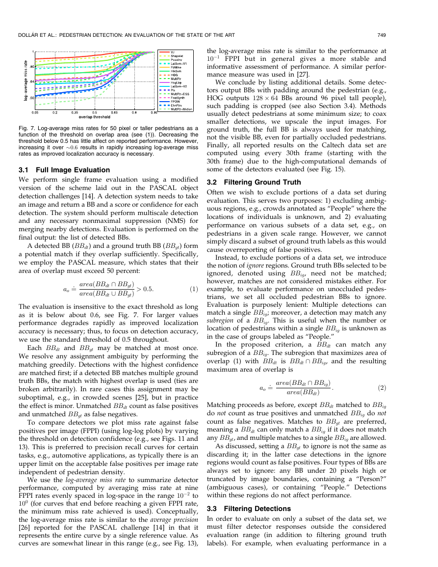
Fig. 7. Log-average miss rates for 50 pixel or taller pedestrians as a
function of the threshold on overlap area (see (1)). Decreasing the
threshold below 0.5 has little affect on reported performance. However,
increasing it over �0:6 results in rapidly increasing log-average miss
rates as improved localization accuracy is necessary.
3.1 Full Image Evaluation
We perform single frame evaluation using a modified
version of the scheme laid out in the PASCAL object
detection challenges [14]. A detection system needs to take
an image and return a BB and a score or confidence for each
detection. The system should perform multiscale detection
and any necessary nonmaximal suppression (NMS) for
merging nearby detections. Evaluation is performed on the
final output: the list of detected BBs.
A detected BB (BBdt) and a ground truth BB (BBgt) form
a potential match if they overlap sufficiently. Specifically,
we employ the PASCAL measure, which states that their
area of overlap must exceed 50 percent:
ao ¼: areaðBBdt \ BBgtÞ
areaðBBdt [ BBgtÞ > 0:5:
ð1Þ
The evaluation is insensitive to the exact threshold as long
as it is below about 0.6, see Fig. 7. For larger values
performance degrades rapidly as improved localization
accuracy is necessary; thus, to focus on detection accuracy,
we use the standard threshold of 0.5 throughout.
Each BBdt and BBgt may be matched at most once.
We resolve any assignment ambiguity by performing the
matching greedily. Detections with the highest confidence
are matched first; if a detected BB matches multiple ground
truth BBs, the match with highest overlap is used (ties are
broken arbitrarily). In rare cases this assignment may be
suboptimal, e.g., in crowded scenes [25], but in practice
the effect is minor. Unmatched BBdt count as false positives
and unmatched BBgt as false negatives.
To compare detectors we plot miss rate against false
positives per image (FPPI) (using log-log plots) by varying
the threshold on detection confidence (e.g., see Figs. 11 and
13). This is preferred to precision recall curves for certain
tasks, e.g., automotive applications, as typically there is an
upper limit on the acceptable false positives per image rate
independent of pedestrian density.
We use the log-average miss rate to summarize detector
performance, computed by averaging miss rate at nine
FPPI rates evenly spaced in log-space in the range 10�2 to
100 (for curves that end before reaching a given FPPI rate,
the minimum miss rate achieved is used). Conceptually,
the log-average miss rate is similar to the average precision
[26] reported for the PASCAL challenge [14] in that it
represents the entire curve by a single reference value. As
curves are somewhat linear in this range (e.g., see Fig. 13),
�
750
IEEE TRANSACTIONS ON PATTERN ANALYSIS AND MACHINE INTELLIGENCE, VOL. 34, NO. 4, APRIL 2012
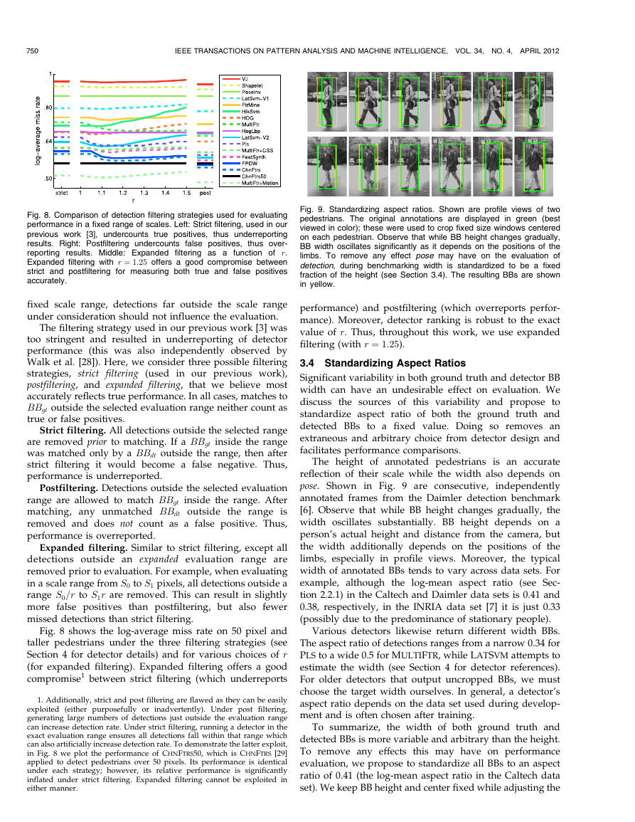
Fig. 8. Comparison of detection filtering strategies used for evaluating
performance in a fixed range of scales. Left: Strict filtering, used in our
previous work [3], undercounts true positives,
thus underreporting
results. Right: Postfiltering undercounts false positives,
thus over-
reporting results. Middle: Expanded filtering as a function of r.
Expanded filtering with r ¼ 1:25 offers a good compromise between
strict and postfiltering for measuring both true and false positives
accurately.
Fig. 9. Standardizing aspect ratios. Shown are profile views of two
pedestrians. The original annotations are displayed in green (best
viewed in color); these were used to crop fixed size windows centered
on each pedestrian. Observe that while BB height changes gradually,
BB width oscillates significantly as it depends on the positions of the
limbs. To remove any effect pose may have on the evaluation of
detection, during benchmarking width is standardized to be a fixed
fraction of the height (see Section 3.4). The resulting BBs are shown
in yellow.
fixed scale range, detections far outside the scale range
under consideration should not influence the evaluation.
The filtering strategy used in our previous work [3] was
too stringent and resulted in underreporting of detector
performance (this was also independently observed by
Walk et al. [28]). Here, we consider three possible filtering
strategies, strict
filtering (used in our previous work),
postfiltering, and expanded filtering, that we believe most
accurately reflects true performance. In all cases, matches to
BBgt outside the selected evaluation range neither count as
true or false positives.
Strict filtering. All detections outside the selected range
are removed prior to matching. If a BBgt inside the range
was matched only by a BBdt outside the range, then after
strict filtering it would become a false negative. Thus,
performance is underreported.
Postfiltering. Detections outside the selected evaluation
range are allowed to match BBgt inside the range. After
matching, any unmatched BBdt outside the range is
removed and does not count as a false positive. Thus,
performance is overreported.
Expanded filtering. Similar to strict filtering, except all
detections outside an expanded evaluation range are
removed prior to evaluation. For example, when evaluating
in a scale range from S0 to S1 pixels, all detections outside a
range S0=r to S1r are removed. This can result in slightly
more false positives than postfiltering, but also fewer
missed detections than strict filtering.
Fig. 8 shows the log-average miss rate on 50 pixel and
taller pedestrians under the three filtering strategies (see
Section 4 for detector details) and for various choices of r
(for expanded filtering). Expanded filtering offers a good
compromise1 between strict filtering (which underreports
1. Additionally, strict and post filtering are flawed as they can be easily
filtering,
exploited (either purposefully or inadvertently). Under post
generating large numbers of detections just outside the evaluation range
can increase detection rate. Under strict filtering, running a detector in the
exact evaluation range ensures all detections fall within that range which
can also artificially increase detection rate. To demonstrate the latter exploit,
in Fig. 8 we plot the performance of CHNFTRS50, which is CHNFTRS [29]
applied to detect pedestrians over 50 pixels. Its performance is identical
under each strategy; however,
its relative performance is significantly
inflated under strict filtering. Expanded filtering cannot be exploited in
either manner.
performance) and postfiltering (which overreports perfor-
mance). Moreover, detector ranking is robust to the exact
value of r. Thus, throughout this work, we use expanded
filtering (with r ¼ 1:25).
3.4 Standardizing Aspect Ratios
Significant variability in both ground truth and detector BB
width can have an undesirable effect on evaluation. We
discuss the sources of this variability and propose to
standardize aspect ratio of both the ground truth and
detected BBs to a fixed value. Doing so removes an
extraneous and arbitrary choice from detector design and
facilitates performance comparisons.
The height of annotated pedestrians is an accurate
reflection of their scale while the width also depends on
pose. Shown in Fig. 9 are consecutive,
independently
annotated frames from the Daimler detection benchmark
[6]. Observe that while BB height changes gradually, the
width oscillates substantially. BB height depends on a
person’s actual height and distance from the camera, but
the width additionally depends on the positions of the
limbs, especially in profile views. Moreover, the typical
width of annotated BBs tends to vary across data sets. For
example, although the log-mean aspect ratio (see Sec-
tion 2.2.1) in the Caltech and Daimler data sets is 0.41 and
0.38, respectively, in the INRIA data set [7] it is just 0.33
(possibly due to the predominance of stationary people).
Various detectors likewise return different width BBs.
The aspect ratio of detections ranges from a narrow 0.34 for
PLS to a wide 0.5 for MULTIFTR, while LATSVM attempts to
estimate the width (see Section 4 for detector references).
For older detectors that output uncropped BBs, we must
choose the target width ourselves. In general, a detector’s
aspect ratio depends on the data set used during develop-
ment and is often chosen after training.
To summarize, the width of both ground truth and
detected BBs is more variable and arbitrary than the height.
To remove any effects this may have on performance
evaluation, we propose to standardize all BBs to an aspect
ratio of 0.41 (the log-mean aspect ratio in the Caltech data
set). We keep BB height and center fixed while adjusting the
�



 2023年江西萍乡中考道德与法治真题及答案.doc
 2012年重庆南川中考生物真题及答案.doc
 2013年江西师范大学地理学综合及文艺理论基础考研真题.doc
 2020年四川甘孜小升初语文真题及答案I卷.doc
 2020年注册岩土工程师专业基础考试真题及答案.doc
 2023-2024学年福建省厦门市九年级上学期数学月考试题及答案.doc
 2021-2022学年辽宁省沈阳市大东区九年级上学期语文期末试题及答案.doc
 2022-2023学年北京东城区初三第一学期物理期末试卷及答案.doc
 2018上半年江西教师资格初中地理学科知识与教学能力真题及答案.doc
 2012年河北国家公务员申论考试真题及答案-省级.doc
 2020-2021学年江苏省扬州市江都区邵樊片九年级上学期数学第一次质量检测试题及答案.doc
 2022下半年黑龙江教师资格证中学综合素质真题及答案.doc