From: AAAI-02 Proceedings. Copyright © 2002, AAAI (www.aaai.org). All rights reserved.
FastSLAM: A Factored Solution to the Simultaneous
Localization and Mapping Problem
Michael Montemerlo and Sebastian Thrun
Daphne Koller and Ben Wegbreit
School of Computer Science
Carnegie Mellon University
Pittsburgh, PA 15213
Computer Science Department
Stanford University
Stanford, CA 94305-9010
mmde@cs.cmu.edu, thrun@cs.cmu.edu
koller@cs.stanford.edu, ben@wegbreit.com
Abstract
The ability to simultaneously localize a robot and ac-
curately map its surroundings is considered by many to
be a key prerequisite of truly autonomous robots. How-
ever, few approaches to this problem scale up to handle
the very large number of landmarks present in real envi-
ronments. Kalman filter-based algorithms, for example,
require time quadratic in the number of landmarks to in-
corporate each sensor observation. This paper presents
FastSLAM, an algorithm that recursively estimates the
full posterior distribution over robot pose and landmark
locations, yet scales logarithmically with the number of
landmarks in the map. This algorithm is based on an ex-
act factorization of the posterior into a product of con-
ditional landmark distributions and a distribution over
robot paths. The algorithm has been run successfully
on as many as 50,000 landmarks, environments far be-
yond the reach of previous approaches. Experimental
results demonstrate the advantages and limitations of
the FastSLAM algorithm on both simulated and real-
world data.
Introduction
The problem of simultaneous localization and mapping, also
known as SLAM, has attracted immense attention in the mo-
bile robotics literature. SLAM addresses the problem of
building a map of an environment from a sequence of land-
mark measurements obtained from a moving robot. Since
robot motion is subject to error, the mapping problem neces-
sarily induces a robot localization problem—hence the name
SLAM. The ability to simultaneously localize a robot and
accurately map its environment is considered by many to be
a key prerequisite of truly autonomous robots [3, 7, 17].
The dominant approach to the SLAM problem was in-
troduced in a seminal paper by Smith, Self, and Cheese-
man [16]. This paper proposed the use of the extended
Kalman filter (EKF) for incrementally estimating the poste-
rior distribution over robot pose along with the positions of
the landmarks. In the last decade, this approach has found
widespread acceptance in field robotics, as a recent tutorial
paper [2] documents. Recent research has focused on scal-
ing this approach to larger environments with more than a
Copyright c 2002, American Association for Artificial Intelli-
gence (www.aaai.org). All rights reserved.
few hundred landmarks [6, 8, 9] and to algorithms for han-
dling data association problems [18].
A key limitation of EKF-based approaches is their compu-
tational complexity. Sensor updates require time quadratic
in the number of landmarks K to compute. This complex-
ity stems from the fact that the covariance matrix maintained
by the Kalman filters has O(K 2) elements, all of which must
be updated even if just a single landmark is observed. The
quadratic complexity limits the number of landmarks that
can be handled by this approach to only a few hundred—
whereas natural environment models frequently contain mil-
lions of features. This shortcoming has long been recog-
nized by the research community [6, 8, 15].
In this paper we approach the SLAM problem from a
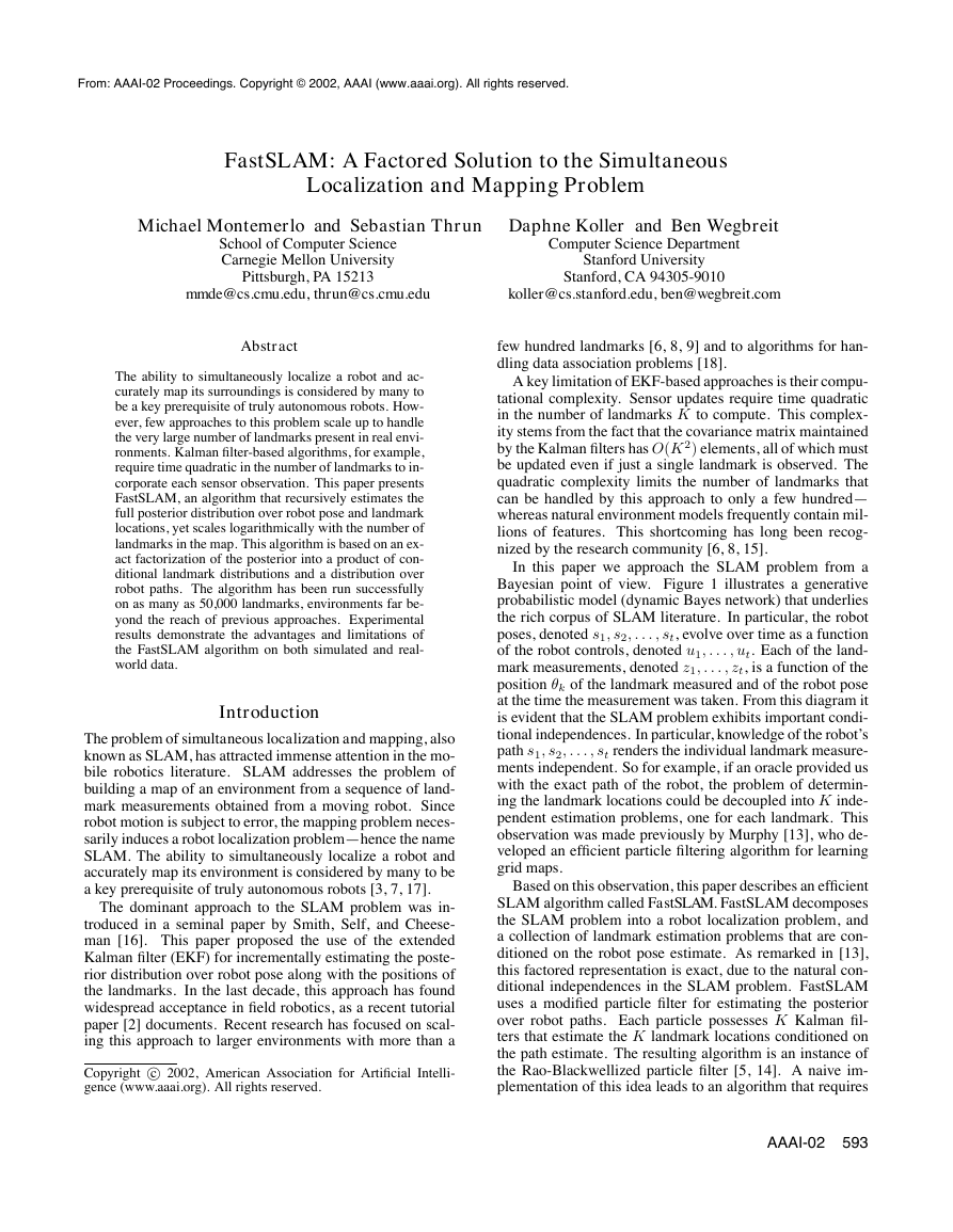
Bayesian point of view. Figure 1 illustrates a generative
probabilistic model (dynamic Bayes network) that underlies
the rich corpus of SLAM literature. In particular, the robot
poses, denoted s1, s2, . . . , st, evolve over time as a function
of the robot controls, denoted u1, . . . , ut. Each of the land-
mark measurements, denoted z1, . . . , zt, is a function of the
position θk of the landmark measured and of the robot pose
at the time the measurement was taken. From this diagram it
is evident that the SLAM problem exhibits important condi-
tional independences. In particular, knowledge of the robot’s
path s1, s2, . . . , st renders the individual landmark measure-
ments independent. So for example, if an oracle provided us
with the exact path of the robot, the problem of determin-
ing the landmark locations could be decoupled into K inde-
pendent estimation problems, one for each landmark. This
observation was made previously by Murphy [13], who de-
veloped an efficient particle filtering algorithm for learning
grid maps.
Based on this observation, this paper describes an efficient
SLAM algorithm called FastSLAM. FastSLAM decomposes
the SLAM problem into a robot localization problem, and
a collection of landmark estimation problems that are con-
ditioned on the robot pose estimate. As remarked in [13],
this factored representation is exact, due to the natural con-
ditional independences in the SLAM problem. FastSLAM
uses a modified particle filter for estimating the posterior
over robot paths. Each particle possesses K Kalman fil-
ters that estimate the K landmark locations conditioned on
the path estimate. The resulting algorithm is an instance of
the Rao-Blackwellized particle filter [5, 14]. A naive im-
plementation of this idea leads to an algorithm that requires
AAAI-02 593
�
1
s1
s
s
. . .
s
2
Figure 1: The SLAM problem: The robot moves from pose s1
through a sequence of controls, u1, u2, . . . , ut. As it moves, it
observes nearby landmarks. At time t = 1, it observes landmark
θ1 out of two landmarks, fθ1, θ2g. The measurement is denoted z1
(range and bearing). At time t = 1, it observes the other landmark,
θ2, and at time t = 3, it observes θ1 again. The SLAM problem is
concerned with estimating the locations of the landmarks and the
robot’s path from the controls u and the measurements z. The gray
shading illustrates a conditional independence relation.
O(M K) time, where M is the number of particles in the
particle filter and K is the number of landmarks. We de-
velop a tree-based data structure that reduces the running
time of FastSLAM to O(M log K), making it significantly
faster than existing EKF-based SLAM algorithms. We also
extend the FastSLAM algorithm to situations with unknown
data association and unknown number of landmarks, show-
ing that our approach can be extended to the full range of
SLAM problems discussed in the literature.
Experimental results using a physical robot and a robot
simulator illustrate that the FastSLAM algorithm can han-
dle orders of magnitude more landmarks than present day
approaches. We also find that in certain situations, an in-
creased number of landmarks K leads to a mild reduction
of the number of particles M needed to generate accurate
maps—whereas in others the number of particles required
for accurate mapping may be prohibitively large.
SLAM Problem Definition
The SLAM problem, as defined in the rich body of litera-
ture on SLAM, is best described as a probabilistic Markov
chain. The robot’s pose at time t will be denoted st. For
robots operating in the plane—which is the case in all of our
experiments—poses are comprised of a robot’s x-y coordi-
nate in the plane and its heading direction.
ferred to as the motion model:
Poses evolve according to a probabilistic law, often re-
p(st j ut, st−1)
(1)
Thus, st is a probabilistic function of the robot control ut
and the previous pose st−1. In mobile robotics, the motion
model is usually a time-invariant probabilistic generalization
of robot kinematics [1].
The robot’s environment possesses K immobile land-
marks. Each landmark is characterized by its location in
space, denoted θk for k = 1, . . . , K. Without loss of gen-
erality, we will think of landmarks as points in the plane, so
that locations are specified by two numerical values.
To map its environment, the robot can sense landmarks.
For example, it may be able to measure range and bearing to
594 AAAI-02
a landmark, relative to its local coordinate frame. The mea-
surement at time t will be denoted zt. While robots can often
sense more than one landmark at a time, we follow com-
monplace notation by assuming that sensor measurements
correspond to exactly one landmark [2]. This convention is
adopted solely for mathematical convenience. It poses no
restriction, as multiple landmark sightings at a single time
step can be processed sequentially.
often referred to as the measurement model:
Sensor measurements are governed by a probabilistic law,
p(zt j st, θ, nt)
(2)
Here θ = fθ1, . . . , θkg is the set of all landmarks, and
nt 2 f1, . . . , Kg is the index of the landmark perceived at
time t. For example, in Figure 1, we have n1 = 1, n2 = 2,
and n3 = 1, since the robot first observes landmark θ1,
then landmark θ2, and finally landmark θ1 for a second time.
Many measurement models in the literature assume that the
robot can measure range and bearing to landmarks, con-
founded by measurement noise. The variable nt is often
referred to as correspondence. Most theoretical work in the
literature assumes knowledge of the correspondence or, put
differently, that landmarks are uniquely identifiable. Practi-
cal implementations use maximum likelihood estimators for
estimating the correspondence on-the-fly, which work well
if landmarks are spaced sufficiently far apart. In large parts
of this paper we will simply assume that landmarks are iden-
tifiable, but we will also discuss an extension that estimates
the correspondences from data.
We are now ready to formulate the SLAM problem. Most
generally, SLAM is the problem of determining the location
of all landmarks θ and robot poses st from measurements
zt = z1, . . . , zt and controls ut = u1, . . . , ut. In probabilis-
tic terms, this is expressed by the posterior p(st, θ j zt, ut),
where we use the superscript t to refer to a set of variables
from time 1 to time t. If the correspondences are known, the
SLAM problem is simpler:
p(st, θ j zt, ut, nt)
(3)
As discussed in the introduction, all individual landmark es-
timation problems are independent if one knew the robot’s
path st and the correspondence variables nt. This condi-
tional independence is the basis of the FastSLAM algorithm
described in the next section.
FastSLAM with Known Correspondences
We begin our consideration with the important case where
the correspondences nt = n1, . . . , nt are known, and so is
the number of landmarks K observed thus far.
Factored Representation
The conditional independence property of the SLAM prob-
lem implies that the posterior (3) can be factored as follows:
p(st, θ j zt, ut, nt)
= p(st j zt, ut, nt)
p(θk j st, zt, ut, nt)
(4)
k
Put verbally, the problem can be decomposed into K+1 esti-
mation problems, one problem of estimating a posterior over
robot paths st, and K problems of estimating the locations
q
q
�
of the K landmarks conditioned on the path estimate. This
factorization is exact and always applicable in the SLAM
problem, as previously argued in [13].
The FastSLAM algorithm implements the path estimator
p(st j zt, ut, nt) using a modified particle filter [4]. As we
argue further below, this filter can sample efficiently from
this space, providing a good approximation of the poste-
rior even under non-linear motion kinematics. The land-
mark pose estimators p(θk j st, zt, ut, nt) are realized by
Kalman filters, using separate filters for different landmarks.
Because the landmark estimates are conditioned on the path
estimate, each particle in the particle filter has its own, lo-
cal landmark estimates. Thus, for M particles and K land-
marks, there will be a total of KM Kalman filters, each of
dimension 2 (for the two landmark coordinates). This repre-
sentation will now be discussed in detail.
Particle Filter Path Estimation
FastSLAM employs a particle filter for estimating the path
posterior p(st j zt, ut, nt) in (4), using a filter that is similar
(but not identical) to the Monte Carlo localization (MCL)
algorithm [1]. MCL is an application of particle filter to
the problem of robot pose estimation (localization). At each
point in time, both algorithms maintain a set of particles rep-
resenting the posterior p(st j zt, ut, nt), denoted St. Each
particle st,[m] 2 St represents a “guess” of the robot’s path:
(5)
We use the superscript notation [m] to refer to the m-th par-
ticle in the set.
The particle set St is calculated incrementally, from the
set St−1 at time t−1, a robot control ut, and a measurement
zt. First, each particle st,[m] in St−1 is used to generate a
probabilistic guess of the robot’s pose at time t
St = fst,[m]gm = fs[m]
t gm
, . . . , s[m]
, s[m]
1
2
s[m]
t
p(st j ut, s[m]
t−1),
(6)
obtained by sampling from the probabilistic motion model.
This estimate is then added to a temporary set of parti-
cles, along with the path st−1,[m]. Under the assumption
that the set of particles in St−1 is distributed according to
p(st−1 j zt−1, ut−1, nt−1) (which is an asymptotically cor-
rect approximation), the new particle is distributed accord-
ing to p(st j zt−1, ut, nt−1). This distribution is commonly
referred to as the proposal distribution of particle filtering.
After generating M particles in this way, the new set St is
obtained by sampling from the temporary particle set. Each
particle st,[m] is drawn (with replacement) with a probability
proportional to a so-called importance factor w[m]
, which is
calculated as follows [10]:
t
p(st,[m] j zt, ut, nt)
target distribution
w[m]
=
t =
proposal distribution
p(st,[m] j zt−1, ut, nt−1)
The exact calculation of (7) will be discussed further below.
The resulting sample set St is distributed according to an ap-
proximation to the desired pose posterior p(st j zt, ut, nt),
an approximation which is correct as the number of particles
M goes to infinity. We also notice that only the most recent
robot pose estimate s[m]
t−1 is used when generating the parti-
cle set St. This will allows us to silently “forget” all other
(7)
pose estimates, rendering the size of each particle indepen-
dent of the time index t.
Landmark Location Estimation
FastSLAM represents the conditional landmark estimates
p(θk j st, zt, ut, nt) in (4) by Kalman filters. Since this
estimate is conditioned on the robot pose, the Kalman filters
are attached to individual pose particles in St. More specifi-
cally, the full posterior over paths and landmark positions in
the FastSLAM algorithm is represented by the sample set
St = fst,[m], µ[m]
1
, Σ[m]
1
, . . . , µ[m]
K , Σ[m]
K gm
(8)
k
k
k
(9)
and Σ[m]
is a two-element vector, and Σ[m]
Here µ[m]
are mean and covariance of the Gaus-
sian representing the k-th landmark θk, attached to the m-th
particle. In the planar robot navigation scenario, each mean
µ[m]
k
The posterior over the k-th landmark pose θk is easily ob-
tained. Its computation depends on whether or not nt = k,
that is, whether or not θk was observed at time t. For nt = k,
we obtain
is a 2 by 2 matrix.
p(θk j st, zt, ut, nt)
Bayes/ p(zt j θk, st, zt−1, ut, nt) p(θk j st, zt−1, ut, nt)
Markov= p(zt j θk, st, nt) p(θk j st−1, zt−1, ut−1, nt−1)
For nt 6= k, we simply leave the Gaussian unchanged:
p(θk j st, zt, ut, nt) = p(θk j st−1, zt−1, ut−1, nt−1) (10)
The FastSLAM algorithm implements the update equation
(9) using the extended Kalman filter (EKF). As in existing
EKF approaches to SLAM, this filter uses a linearized ver-
j st, θ, nt) [2]. Thus,
sion of the perceptual model p(zt
FastSLAM’s EKF is similar to the traditional EKF for
SLAM [16] in that it approximates the measurement model
using a linear Gaussian function. We note that, with a lin-
ear Gaussian observation model, the resulting distribution
p(θk j st, zt, ut, nt) is exactly a Gaussian, even if the mo-
tion model is not linear. This is a consequence of the use
of sampling to approximate the distribution over the robot’s
pose.
One significant difference between the FastSLAM algo-
rithm’s use of Kalman filters and that of the traditional
SLAM algorithm is that the updates in the FastSLAM algo-
rithm involve only a Gaussian of dimension two (for the two
landmark location parameters), whereas in the EKF-based
SLAM approach a Gaussian of size 2K+3 has to be updated
(with K landmarks and 3 robot pose parameters). This cal-
culation can be done in constant time in FastSLAM, whereas
it requires time quadratic in K in standard SLAM.
Calculating the Importance Weights
Let us now return to the problem of calculating the impor-
tance weights w[m]
needed for particle filter resampling, as
defined in (7):
p(st,[m] j zt, ut, nt)
t
w[m]
t
/
p(st,[m] j zt−1, ut, nt−1)
p(zt, nt j st,[m], zt−1, ut, nt−1)
p(zt, nt j zt−1, ut, nt−1)
Bayes=
AAAI-02 595
�
k £ 4 ?
k £ 4 ?
F
F
T
T
k £ 2 ?
k £ 2 ?
k £ 6 ?
k £ 6 ?
T
T
F
F
T
T
F
F
k £ 1 ?
k £ 1 ?
k £ 3 ?
k £ 3 ?
k £ 5 ?
k £ 5 ?
k £ 7 ?
k £ 7 ?
T
T
F
F
T
T
[m]
[m]
1,S
1,S
[m]
[m]
1
1
[m]
[m]
2,S
2,S
[m]
[m]
2
2
[m]
[m]
3,S
3,S
[m]
[m]
3
3
F
F
[m]
[m]
4,S
4,S
T
T
F
F
T
T
F
F
[m]
[m]
4
4
[m]
[m]
5,S
5,S
[m]
[m]
5
5
[m]
[m]
6,S
6,S
[m]
[m]
6
6
[m]
[m]
7,S
7,S
[m]
[m]
7
7
[m]
[m]
8,S
8,S
[m]
[m]
8
8
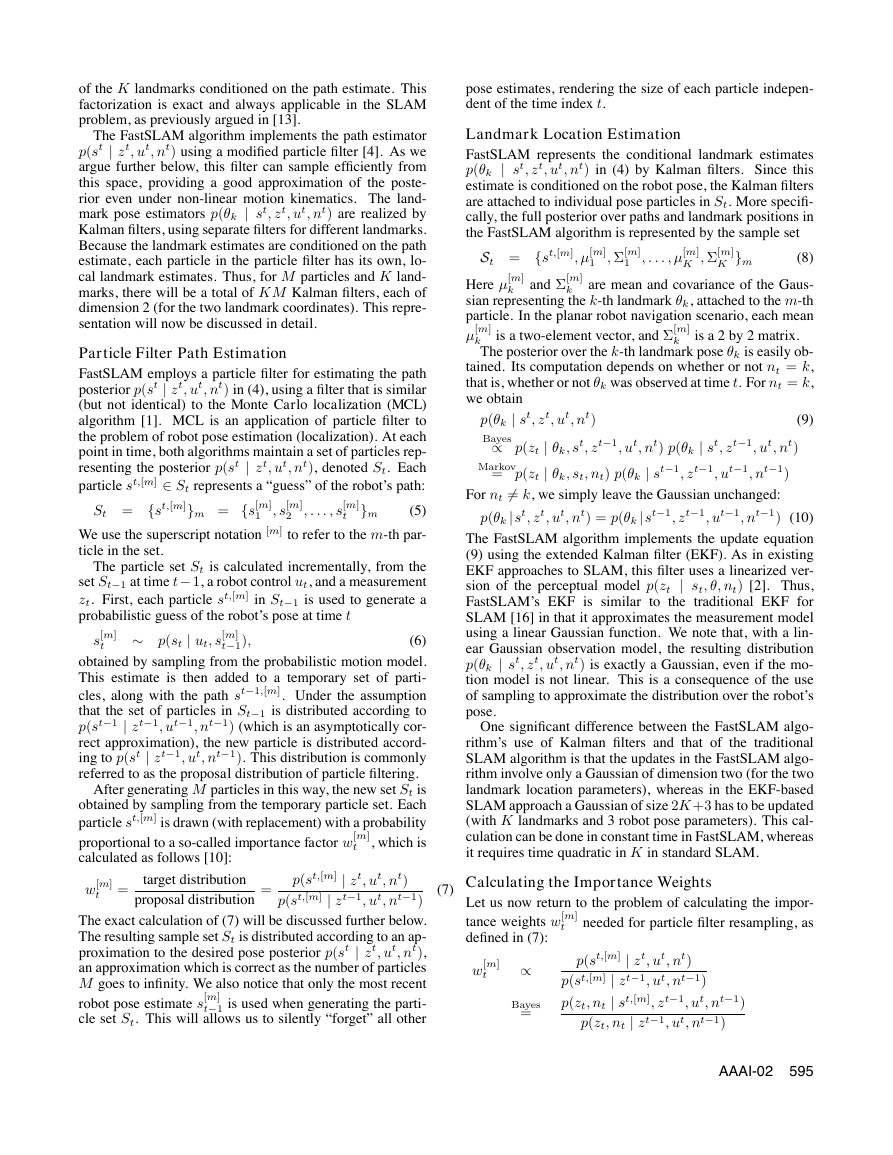
Figure 2: A tree representing K = 8 landmark estimates within a
single particle.
p(st,[m] j zt−1, ut, nt)
p(st,[m] j zt−1, ut, nt)
p(zt, nt j zt−1, ut, nt−1)
p(zt, nt j st,[m], zt−1, ut, nt−1)
p(zt, nt j st,[m], zt−1, ut, nt−1)
p(zt, nt j θ, st,[m], zt−1, ut, nt−1)
p(θ j st,[m], zt−1, ut, nt) dθ
t
)
, nt) p(nt j θ, s[m]
p(zt, nt j θ, s[m]
p(θ j st−1,[m], zt−1, ut−1, nt−1) dθ
p(zt j θ, s[m]
p(θ j st−1,[m], zt−1, ut−1, nt−1) dθ
p(zt j θ, s[m]
p(θ j st−1,[m], zt−1, ut−1, nt−1) dθ
p(zt j θ[m]
, nt) p(θ[m]
nt ) dθnt
, s[m]
, nt)
nt
)
t
t
t
t
(11)
=
/
=
Markov=
=
/
EKF
j θ, s[m]
Here we assume that the distribution p(nt
) is
uniform—a common assumption in SLAM. In the last line,
“EKF” makes explicit the use of a linearized model as an ap-
proximation to the observation model p(zt j θ[m]
), and
the resulting Gaussian posterior p(θ[m]
nt ). The final integra-
tion is easily calculated in closed form for a linear Gaussian.
nt , s[m]
t
t
Efficient Implementation
The FastSLAM algorithm, as described thus far, may require
time linear in the number of landmarks K for each update
iteration if implemented naively. This is because of the re-
sampling step; every time a particle is added to St, its has
to be copied. Since each particle contains K landmark esti-
mates, this copying procedure requires O(M K) time. How-
ever, most of this copying can be avoided.
Our approach makes it possible to execute a FastSLAM
iteration in O(M log K) time. The basic idea is that the set
of Gaussians in each particle is represented by a balanced bi-
nary tree. Figure 2 shows such a tree for a single particle, in
the case of 8 landmarks. The Gaussian parameters µ[m]
and
Σ[m]
are located at the leaves of the tree. Clearly, accessing
k
k
596 AAAI-02
T
T
k £ 4 ?
k £ 4 ?
F
F
k £ 2 ?
k £ 2 ?
F
F
T
T
k £ 3 ?
k £ 3 ?
F
F
T
T
3,S
3,S
[m]
[m]
[m]
[m]
3
3
new particle
new particle
k £ 4 ?
k £ 4 ?
k £ 4 ?
k £ 4 ?
k £ 4 ?
k £ 4 ?
k £ 4 ?
F
F
F
F
F
F
F
T
T
T
T
T
T
T
old particle
old particle
k £ 2 ?
k £ 2 ?
k £ 2 ?
k £ 2 ?
k £ 2 ?
k £ 2 ?
k £ 2 ?
T
T
T
T
T
T
T
F
F
F
F
F
F
F
k £ 6 ?
k £ 6 ?
k £ 6 ?
k £ 6 ?
k £ 6 ?
k £ 6 ?
k £ 6 ?
T
T
T
T
T
T
T
F
F
F
F
F
F
F
k £ 1 ?
k £ 1 ?
k £ 1 ?
k £ 1 ?
k £ 1 ?
k £ 1 ?
k £ 1 ?
k £ 3 ?
k £ 3 ?
k £ 3 ?
k £ 3 ?
k £ 3 ?
k £ 3 ?
k £ 3 ?
k £ 1 ?
k £ 1 ?
k £ 1 ?
k £ 1 ?
k £ 1 ?
k £ 1 ?
k £ 1 ?
k £ 3 ?
k £ 3 ?
k £ 3 ?
k £ 3 ?
k £ 3 ?
k £ 3 ?
k £ 3 ?
T
T
T
T
T
T
T
F
F
F
F
F
F
F
T
T
T
T
T
T
T
F
F
F
F
F
F
F
T
T
T
T
T
T
T
F
F
F
F
F
F
F
T
T
T
T
T
T
T
F
F
F
F
F
F
F
[m]
[m]
[m]
[m]
[m]
[m]
[m]
1,S
1,S
1,S
1,S
1,S
1,S
1,S
[m]
[m]
[m]
[m]
[m]
[m]
[m]
1
1
1
1
1
1
1
[m]
[m]
[m]
[m]
[m]
[m]
[m]
2,S
2,S
2,S
2,S
2,S
2,S
2,S
[m]
[m]
[m]
[m]
[m]
[m]
[m]
2
2
2
2
2
2
2
[m]
[m]
[m]
[m]
[m]
[m]
[m]
3,S
3,S
3,S
3,S
3,S
3,S
3,S
[m]
[m]
[m]
[m]
[m]
[m]
[m]
3
3
3
3
3
3
3
[m]
[m]
[m]
[m]
[m]
[m]
[m]
4,S
4,S
4,S
4,S
4,S
4,S
4,S
[m]
[m]
[m]
[m]
[m]
[m]
[m]
4
4
4
4
4
4
4
[m]
[m]
[m]
[m]
[m]
[m]
[m]
5,S
5,S
5,S
5,S
5,S
5,S
5,S
[m]
[m]
[m]
[m]
[m]
[m]
[m]
5
5
5
5
5
5
5
[m]
[m]
[m]
[m]
[m]
[m]
[m]
6,S
6,S
6,S
6,S
6,S
6,S
6,S
[m]
[m]
[m]
[m]
[m]
[m]
[m]
6
6
6
6
6
6
6
[m]
[m]
[m]
[m]
[m]
[m]
[m]
7,S
7,S
7,S
7,S
7,S
7,S
7,S
[m]
[m]
[m]
[m]
[m]
[m]
[m]
7
7
7
7
7
7
7
[m]
[m]
[m]
[m]
[m]
[m]
[m]
8,S
8,S
8,S
8,S
8,S
8,S
8,S
[m]
[m]
[m]
[m]
[m]
[m]
[m]
8
8
8
8
8
8
8
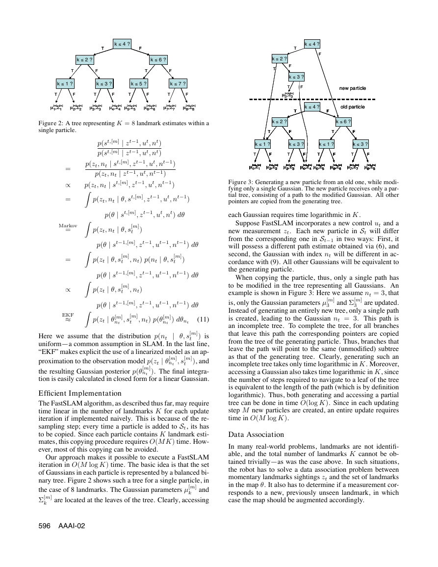
Figure 3: Generating a new particle from an old one, while modi-
fying only a single Gaussian. The new particle receives only a par-
tial tree, consisting of a path to the modified Gaussian. All other
pointers are copied from the generating tree.
each Gaussian requires time logarithmic in K.
Suppose FastSLAM incorporates a new control ut and a
new measurement zt. Each new particle in St will differ
from the corresponding one in St−1 in two ways: First, it
will possess a different path estimate obtained via (6), and
second, the Gaussian with index nt will be different in ac-
cordance with (9). All other Gaussians will be equivalent to
the generating particle.
3
3
and Σ[m]
When copying the particle, thus, only a single path has
to be modified in the tree representing all Gaussians. An
example is shown in Figure 3: Here we assume nt = 3, that
is, only the Gaussian parameters µ[m]
are updated.
Instead of generating an entirely new tree, only a single path
is created, leading to the Gaussian nt = 3. This path is
an incomplete tree. To complete the tree, for all branches
that leave this path the corresponding pointers are copied
from the tree of the generating particle. Thus, branches that
leave the path will point to the same (unmodified) subtree
as that of the generating tree. Clearly, generating such an
incomplete tree takes only time logarithmic in K. Moreover,
accessing a Gaussian also takes time logarithmic in K, since
the number of steps required to navigate to a leaf of the tree
is equivalent to the length of the path (which is by definition
logarithmic). Thus, both generating and accessing a partial
tree can be done in time O(log K). Since in each updating
step M new particles are created, an entire update requires
time in O(M log K).
Data Association
In many real-world problems, landmarks are not identifi-
able, and the total number of landmarks K cannot be ob-
tained trivially—as was the case above. In such situations,
the robot has to solve a data association problem between
momentary landmarks sightings zt and the set of landmarks
in the map θ. It also has to determine if a measurement cor-
responds to a new, previously unseen landmark, in which
case the map should be augmented accordingly.
m
m
m
m
m
m
m
m
m
m
m
m
m
m
m
m
m
m
m
m
m
m
m
m
m
m
m
m
m
m
m
m
m
m
m
m
m
m
m
m
m
m
m
m
m
m
m
m
m
m
m
m
m
m
m
m
m
m
m
m
m
m
m
m
m
m
m
m
m
m
m
m
m
m
�
(a)
(b)
(c)
Figure 4: (a) Physical robot mapping rocks, in a testbed developed for Mars Rover research. (b) Raw range and path data. (c) Map generated
using FastSLAM (dots), and locations of rocks determined manually (circles).
In most existing SLAM solutions based on EKFs, these
problems are solved via maximum likelihood. More specif-
ically, the probability of a data association nt is given by
=
PF
p(nt j zt, ut)
Markov=
m
m
Bayes/
p(nt j st, zt, ut) p(st j zt, ut) dst
p(nt j st,[m], zt, ut)
p(nt j s[m]
p(zt j s[m]
, nt)
, zt)
t
t
(12)
m
The step labeled “PF” uses the particle filter approxima-
tion to the posterior p(st j zt, ut). The final step assumes
a uniform prior p(nt j st), which is commonly used [2].
The maximum likelihood data association is simply the in-
dex nt that maximizes (12).
If the maximum value of
p(nt j zt, ut)—with careful consideration of all constants
in (12)—is below a threshold α, the landmark is considered
previously unseen and the map is augmented accordingly.
t
t
p(ztjs[m]
t = argmaxnt
In FastSLAM, the data association is estimated on a per-
particle basis: n[m]
, nt). As a result,
different particles may rely on different values of n[m]
. They
might even possess different numbers of landmarks in their
respective maps. This constitutes a primary difference to
EKF approaches, which determine the data association only
once for each sensor measurement.
It has been observed
frequently that false data association will make the conven-
tional EKF approach fail catastrophically [2]. FastSLAM is
more likely to recover, thanks to its ability to pursue multi-
ple data associations simultaneously. Particles with wrong
data association are (in expectation) more likely to disap-
pear in the resampling process than those that guess the data
association correctly.
We believe that, under mild assumptions (e.g., minimum
spacing between landmarks and bounded sensor error), the
data association search can be implemented in time loga-
rithmic in N. One possibility is the use of kd-trees as an
indexing scheme in the tree structures above, instead of the
landmark number, as proposed in [11].
Experimental Results
The FastSLAM algorithm was tested extensively under vari-
ous conditions. Real-world experiments were complimented
by systematic simulation experiments,
to investigate the
scaling abilities of the approach. Overall, the results indicate
favorably scaling to large number of landmarks and small
particle sets. A fixed number of particles (e.g., M = 100)
appears to work well across a large number of situations.
Figure 4a shows the physical robot testbed, which consists
of a small arena set up under NASA funding for Mars Rover
research. A Pioneer robot equipped with a SICK laser range
finder was driven along an approximate straight line, gener-
ating the raw data shown in Figure 4b. The resulting map
generated with M = 10 samples is depicted in Figure 4c,
with manually determined landmark locations marked by
circles. The robot’s estimates are indicated by x’s, illustrat-
ing the high accuracy of the resulting maps. FastSLAM re-
sulted in an average residual map error of 8.3 centimeters,
when compared to the manually generated map.
Unfortunately, the physical testbed does not allow for sys-
tematic experiments regarding the scaling properties of the
approach.
In extensive simulations, the number of land-
marks was increased up to a total of 50,000, which Fast-
SLAM successfully mapped with as few as 100 particles.
Here, the number of parameters in FastSLAM is approx-
imately 0.3% of that in the conventional EKF. Maps with
50,000 landmarks are out of range for conventional SLAM
techniques, due to their enormous computational complex-
ity. Figure 5 shows example maps with smaller numbers
of landmarks, for different maximum sensor ranges as indi-
cated. The ellipses in Figure 5 visualize the residual uncer-
tainty when integrated over all particles and Gaussians.
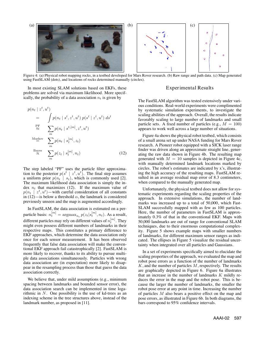
In a set of experiments specifically aimed to elucidate the
scaling properties of the approach, we evaluated the map and
robot pose errors as a function of the number of landmarks
K, and the number of particles M, respectively. The results
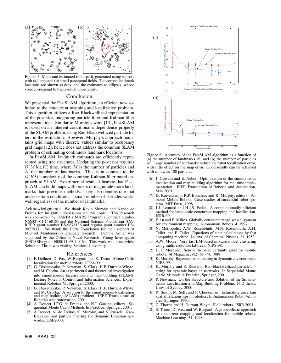
are graphically depicted in Figure 6. Figure 6a illustrates
that an increase in the number of landmarks K mildly re-
duces the error in the map and the robot pose. This is be-
cause the larger the number of landmarks, the smaller the
robot pose error at any point in time. Increasing the number
of particles M also bears a positive effect on the map and
pose errors, as illustrated in Figure 6b. In both diagrams, the
bars correspond to 95% confidence intervals.
AAAI-02 597
�
(a)
(b)
Figure 5: Maps and estimated robot path, generated using sensors
with (a) large and (b) small perceptual fields. The correct landmark
locations are shown as dots, and the estimates as ellipses, whose
sizes correspond to the residual uncertainty.
Conclusion
We presented the FastSLAM algorithm, an efficient new so-
lution to the concurrent mapping and localization problem.
This algorithm utilizes a Rao-Blackwellized representation
of the posterior, integrating particle filter and Kalman filter
representations. Similar to Murphy’s work [13], FastSLAM
is based on an inherent conditional independence property
of the SLAM problem, using Rao-Blackwellized particle fil-
ters in the estimation. However, Murphy’s approach main-
tains grid maps with discrete values similar to occupancy
grid maps [12], hence does not address the common SLAM
problem of estimating continuous landmark locations.
In FastSLAM, landmark estimates are efficiently repre-
sented using tree structures. Updating the posterior requires
O(M log K) time, where M is the number of particles and
K the number of landmarks. This is in contrast to the
O(K 2) complexity of the common Kalman-filter based ap-
proach to SLAM. Experimental results illustrate that Fast-
SLAM can build maps with orders of magnitude more land-
marks than previous methods. They also demonstrate that
under certain conditions, a small number of particles works
well regardless of the number of landmarks.
Acknowledgments We thank Kevin Murphy and Nando de
Freitas for insightful discussions on this topic. This research
was sponsored by DARPA’s MARS Program (Contract number
N66001-01-C-6018) and the National Science Foundation (CA-
REER grant number IIS-9876136 and regular grant number IIS-
9877033). We thank the Hertz Foundation for their support of
Michael Montemerlo’s graduate research. Daphne Koller was
supported by the Office of Naval Research, Young Investigator
(PECASE) grant N00014-99-1-0464. This work was done while
Sebastian Thrun was visiting Stanford University.
References
localization for mobile robots. ICRA-99.
[2] G. Dissanayake, P. Newman, S. Clark, H.F. Durrant-Whyte,
and M. Csorba. An experimental and theoretical investigation
into simultaneous localisation and map building (SLAM).
Lecture Notes in Control and Information Sciences: Exper-
imental Robotics VI, Springer, 2000.
[3] G. Dissanayake, P. Newman, S. Clark, H.F. Durrant-Whyte,
and M. Csorba. A solution to the simultaneous localisation
and map building (SLAM) problem.
IEEE Transactions of
Robotics and Automation, 2001.
[4] A. Doucet, J.F.G. de Freitas, and N.J. Gordon, editors. Se-
quential Monte Carlo Methods In Practice. Springer, 2001.
[5] A Doucet, N. de Freitas, K. Murphy, and S. Russell. Rao-
Blackwellised particle filtering for dynamic Bayesian net-
works. UAI-2000.
Accuracy of FastSLAM as K Increases
Robot Position Error
Landmark Position Error
10
50
100
500
1000
5000
Number of landmarks K
Accuracy of FastSLAM as Number of Particles Increases
Robot Position Error
Landmark Position Error
(a)
(b)
0.9
0.8
0.7
0.6
0.5
0.4
0.3
0.2
2.5
2
1.5
1
0.5
i
)
n
o
i
t
a
v
e
d
d
r
a
d
n
a
t
s
(
r
o
r
r
E
n
o
i
t
i
s
o
P
)
n
o
i
t
i
a
v
e
d
d
r
a
d
n
a
t
s
(
r
o
r
r
E
n
o
i
t
i
s
o
P
0
0
50
100
150
Number of Particles
200
250
Figure 6: Accuracy of the FastSLAM algorithm as a function of
(a) the number of landmarks N, and (b) the number of particles
M. Large number of landmarks reduce the robot localization error,
with little effect on the map error. Good results can be achieved
with as few as 100 particles.
[6] J. Guivant and E. Nebot. Optimization of the simultaneous
localization and map building algorithm for real time imple-
mentation.
IEEE Transaction of Robotic and Automation,
May 2001.
[7] D. Kortenkamp, R.P. Bonasso, and R. Murphy, editors. AI-
based Mobile Robots: Case studies of successful robot sys-
tems, MIT Press, 1998.
[8] J.J. Leonard and H.J.S. Feder. A computationally efficient
method for large-scale concurrent mapping and localization.
ISRR-99.
[9] F. Lu and E. Milios. Globally consistent range scan alignment
for environment mapping. Autonomous Robots, 4, 1997.
[10] N. Metropolis, A.W. Rosenbluth, M.N. Rosenbluth, A.H.
Teller, and E. Teller. Equations of state calculations by fast
computing machine. Journal of Chemical Physics, 21, 1953.
[11] A.W. Moore. Very fast EM-based mixture model clustering
using multiresolution kd-trees. NIPS-98.
[12] H. P. Moravec. Sensor fusion in certainty grids for mobile
robots. AI Magazine, 9(2):61–74, 1988.
NIPS-99.
[14] K. Murphy and S. Russell. Rao-blackwellized particle fil-
tering for dynamic bayesian networks. In Sequential Monte
Carlo Methods in Practice, Springer, 2001.
[15] P. Newman. On the Structure and Solution of the Simulta-
neous Localisation and Map Building Problem. PhD thesis,
Univ. of Sydney, 2000.
[16] R. Smith, M. Self, and P. Cheeseman. Estimating uncertain
spatial relationships in robotics. In Autonomous Robot Vehni-
cles, Springer, 1990.
[17] C. Thorpe and H. Durrant-Whyte. Field robots. ISRR-2001.
[18] S. Thrun, D. Fox, and W. Burgard. A probabilistic approach
to concurrent mapping and localization for mobile robots.
Machine Learning, 31, 1998.
[1] F. Dellaert, D. Fox, W. Burgard, and S. Thrun. Monte Carlo
[13] K. Murphy. Bayesian map learning in dynamic environments.
598 AAAI−02
�



 2023年江西萍乡中考道德与法治真题及答案.doc
 2012年重庆南川中考生物真题及答案.doc
 2013年江西师范大学地理学综合及文艺理论基础考研真题.doc
 2020年四川甘孜小升初语文真题及答案I卷.doc
 2020年注册岩土工程师专业基础考试真题及答案.doc
 2023-2024学年福建省厦门市九年级上学期数学月考试题及答案.doc
 2021-2022学年辽宁省沈阳市大东区九年级上学期语文期末试题及答案.doc
 2022-2023学年北京东城区初三第一学期物理期末试卷及答案.doc
 2018上半年江西教师资格初中地理学科知识与教学能力真题及答案.doc
 2012年河北国家公务员申论考试真题及答案-省级.doc
 2020-2021学年江苏省扬州市江都区邵樊片九年级上学期数学第一次质量检测试题及答案.doc
 2022下半年黑龙江教师资格证中学综合素质真题及答案.doc