2810
IEEE TRANSACTIONS ON CYBERNETICS, VOL. 46, NO. 12, DECEMBER 2016
Event Detection in Twitter Microblogging
Nikolaos D. Doulamis, Member, IEEE, Anastasios D. Doulamis, Member, IEEE, Panagiotis Kokkinos,
and Emmanouel (Manos) Varvarigos
Abstract—The millions of tweets submitted daily overwhelm
users who find it difficult to identify content of interest revealing
the need for event detection algorithms in Twitter. Such algo-
rithms are proposed in this paper covering both short (identifying
what is currently happening) and long term periods (reviewing
the most salient recently submitted events). For both scenarios,
we propose fuzzy represented and timely evolved tweet-based
theoretic information metrics to model Twitter dynamics. The
Riemannian distance is also exploited with respect to words’ sig-
natures to minimize temporal effects due to submission delays.
Events are detected through a multiassignment graph partition-
ing algorithm that: 1) optimally retains maximum coherence
within a cluster and 2) while allowing a word to belong
to several clusters (events). Experimental results on real-life
data demonstrate that our approach outperforms other methods.
Index Terms—Clustering, document and text processing, fuzzy
representation, pattern analysis, tweet characterization.
I. INTRODUCTION
E VENT detection algorithms that identify what is really
being discussed in Twitter are necessary for structuring
micro-blogging content [1]–[3]. The underlying idea of such
algorithms is to extract a set of keywords that show an increas-
ing usage at about the time an event is happening. Two main
steps are required to construct an efficient tweet event detec-
tion algorithm: 1) we need to textually characterize the tweet
content and 2) we need to apply learning strategies to retrieve
events from tweets by analyzing the time evolution of the
appearance count of certain words.
Current information theoretic metrics for document char-
acterization, e.g., the term frequency–inverse document fre-
quency (TF–IDF) [4] or distributional features [5], are not
suitable for Twitter. This is because tweets: 1) are short mes-
sages (no more than 140 characters) leading to statistical
inaccuracies when applying traditional document metrics on
them; 2) present dynamic behavior with large volumes of posts
being published during short time periods; and 3) exhibits
is posted.
temporal shifts at
the times a particular event
Manuscript received May 30, 2015; revised September 2, 2015; accepted
September 27, 2015. Date of publication November 2, 2015; date of cur-
rent version November 15, 2016. This work was supported by the European
Union funded Project 4DCHWORLD through FP7 People Program under
Grant 324523. This paper was recommended by Associate Editor J. Liu.
N. D. Doulamis and A. D. Doulamis are with the National Technical
University of Athens, Athens 157 73, Greece (e-mail: ndoulam@cs.ntua.gr;
adoulam@cs.ntua.gr).
P. Kokkinos and E. Varvarigos are with the Computer Engineering and
Informatics Department, University of Patras, Patras 265 04, Greece (e-mail:
kokkinop@ceid.upatras.gr; manos@ceid.upatras.gr).
Color versions of one or more of the figures in this paper are available
online at http://ieeexplore.ieee.org.
Digital Object Identifier 10.1109/TCYB.2015.2489841
All
Twitter is also characterized by some key features: 1) users
may subscribe to other users’ tweets (followers) and 2) Twitter
has the ability to forward a tweet to their followers (retweets).
these reasons make processing of the tweets’ con-
tent very different than that in traditional document analysis.
Particularly, tweets present different word distributions from
one time period to another, as new trends appear for the dis-
cussed topics. This implies time varying document frequency
metrics. Additionally,
tweets are generated from different
authors having different target audiences and/or writing styles,
and they contain a number of extra symbols, misspelled or
abbreviated words, resulting in a noisy estimation of the term
frequency metric. Finally, Twitter’s following and retweeting
are important and they should be taken into account in the
analysis.
After text characterization, the second step is to extract
events (equivalently sets of keywords) from the tweet posts by
detecting common temporal similarities in their words’ time
series signals; the words of an event present a synchronized
behavior in their appearance count. The research challenges at
this stage are the following.
1) Tweet messages are often of unstructured meanings and
the words of an event do not appear under a synchro-
nized manner. This requires new forms of representation
to compensate for the vagueness introduced by these
temporal variations.
2) In contrast to conventional one-class assignment cluster-
ing methods, multiassignment clustering approaches are
needed, since one word may belong to several events.
3) As words may belong to several events, clustering is not
well-separable requiring the use of advanced methods,
like graph partitioning.
A. Contribution
In this paper, we examine two scenarios. The short-term
event detection (scenario 1) aims at detecting the most salient
events that are currently being posted by the tweets. The long-
term event detection (scenario 2) reviews events that have
occurred over a long time period and aims at synopsizing what
has mostly happened over that period.
For both scenarios, we propose new information metrics that
exploit the dynamic nature of Twitter, and combine a num-
ber of techniques. First, we redefine the IDF score so as to
make it a time varying metric that has the ability to sense
“trending” topics. Second, we introduce conditional scores in
order to address short message inaccuracies. Third, we apply
processing over several time intervals so as to create “fea-
ture trajectories.” Fourth, we propose a fuzzy representation
2168-2267 c 2015 IEEE. Personal use is permitted, but republication/redistribution requires IEEE permission.
See http://www.ieee.org/publications_standards/publications/rights/index.html for more information.
�
DOULAMIS et al.: EVENT DETECTION IN TWITTER MICROBLOGGING
2811
in order to compensate for temporal shifts in tweets’ posting.
Fifth, we model the clustering problem as a multi (instead of
a single) assignment spectral graph partitioning problem.
INDICATIVE STORIES FOR SCENARIO 1 CASE
TABLE I
This paper
is organized as follows. Section II
intro-
duces metrics for tweet characterization. Section III discusses
the multiassignment graph partitioning problem, Section IV
defines the similarity measures. and Section V provides exper-
imental results. Previous works are given in Section VI.
Finally, Section VII concludes the paper.
II. MODELING DYNAMIC NATURE OF TWEETS
A. Problem Formulation
We assume that the event detection algorithm is activated
at the end of the kth time interval (period) (tk−1, tk] = (tk −
β, tk], k = 1, 2, . . . , where β > 0 denotes the duration of the
interval. We let N(k) be the number of tweets that are posted
during the kth time interval. In our setting, M events can be
detected within the kth time interval. Each event is defined as
, i = 1, 2, . . . , Lm} of Lm words, where
a set of W(m) = {wm
m = 1, . . . , M, stands for the event index. Two scenarios are
supported.
i
Scenario 1 (Short-Term Event Detection): Scenario 1
extracts the most important events currently being posted in
Twitter. In this scenario, we need to find out the synchronized
words’ behavior, i.e., which of the words posted by the tweets
present similar temporal patterns.
Scenario 2 (Long-Term Event Detection): Scenario 2
reviews the events that have occurred over a long time interval
to synopsize what has mostly happened during that inter-
val. To detect the most important events in this scenario,
we need to find out similar words’ behavior being invariant
to time shifts and for this reason new similarity metrics are
needed.
To capture the temporal dynamicity of tweets’ content, we
form feature trajectories that model words’ distribution over
a time period. Let us denote by sw(k) the feature trajec-
tory of a word w. In scenario 1, the purpose is to cluster
words together that present similar burst patterns in their dis-
tribution. Thus, we consider the similarity D(swi(k), swj(k))
of two words’ feature trajectories. Instead, scenario 2 syn-
opsizes what has mostly happened in long-time periods and
therefore the words’ distributions are clustered together inde-
pendently of whether they are shifted in time, thus optimizing
D(swi(k + t), swj(k)) for every time shift t of the feature time
signal.
Table I presents indicative stories extracted from tweets
posted on specific time instances. These tweets were retrieved
by querying Twitter using the keywords of “BBC sports,”
“BBC auto,” and “BBC news.” The purpose of our algorithm
for scenario 1 is to identify the most important events posted
on Twitter at the specific time, by clustering the keywords
these events are composed of. Table II presents indicative key-
words related to events occurring over longer time periods
(e.g., half a month). Again, these tweets have been retrieved
by querying Twitter using the keyword of BBC news. Since
scenario 2 synopsizes what has mostly happened during longer
INDICATIVE STORIES FOR SCENARIO 2 CASE
TABLE II
time periods, in Table II, we present only the relevant key-
words of the main stories. From a technical point of view,
the main difficulty in the scenario 2 case is that the relevant
keywords are not absolutely synchronized and they are noisy.
To cope with this, the Riemannian similarity metric is used to
compensate micro-variations in words’ signals.
B. Tweet-Based Information Theoretic Metrics
The TF–IDF [4] metric is not suitable to characterize
tweets content. First, tweets are very short messages which
lead to statistical inaccuracies in calculating TF scores. One
way to compensate this difficulty is to consider as a docu-
ment a collection of tweets gathered over a time interval k,
instead of a single tweet. However, since tweets are posted
by different authors of different target objectives, or writ-
ing styles, conditional probability distributions need to be
incorporated. Additionally, we propose metrics that also con-
sider Twitter-specific features such as retweeting and num-
ber of followers. Second, Twitter is very dynamic. This
implies that words that are not statistically frequent in pre-
vious time intervals may be common in the current ones,
since users’ trends evolve through time. This transforms the
IDF score to a time varying variable measuring the inverse
trend frequency (ITF) of a word proportionally to IDF that
measures the IDF. Third, there are usually temporal delays
when posting tweets. Thus, event detection is very sensitive
to those time shifts (temporal variations). Consequently, it
is not proper to estimate the tweets metrics independently
from one time interval to another, but instead the score of
one time interval should affect the scores of adjacent inter-
vals. To address this, fuzzy theoretic information metrics are
adopted.
1) Conditional Word Tweet Frequency–Inverse Trend Word
Tweet Frequency: We denote by N(w)(k) the number of
�
2812
IEEE TRANSACTIONS ON CYBERNETICS, VOL. 46, NO. 12, DECEMBER 2016
ITWTF(k, p, w) = log
i=1 N(k − i)
p
i=1 N(w)(k − i)
p
.
(2)
ϑ3(k, w)
tweets containing the word w over all the N(k) tweets col-
lected at
time interval k. We define the conditional word
tweet frequency (CWTF) at time instance k and for a given
word w as
CWTF(k, w) = N(w)(k)/N(k).
(1)
The main difference of CWTF from the classical description
of TF is that, here we count the number of tweets that contain
a specific word within the current examined time interval k
instead of counting the number of times that a word appears
within a document. That is, all tweets that contain the specific
word contribute the same to the calculation of CWTF. Thus,
CWTF models a conditional distribution of
tweets fre-
quency,
they contain
i.e.,
tweets under the condition that
the word w.
We define the inverse trend word tweet frequency (ITWTF)
as a metric that assesses how frequently tweet posts contain
the specific word w over p previous time intervals, (tk−1 −
β, tk−1], . . . , (tk−p − β, tk−p]. In particular, we have that
In contrast to the conventional IDF score, ITWTF is a time
varying metric that evolves as new time intervals are taken
into account. A word that is rarely frequent up to the cur-
rent examined time interval k will receive high values of
ITWTF. However, if this word becomes trendy at the current
time interval k, the CWTF score will take high values, forcing
the product CWTF*ITWTF to be high. As long as this word
remains trendy, in the forthcoming time intervals the ITWTF
score will start to decay forcing the product CWTF*ITWTF
to start decreasing as well. This means that, events that
have been extracted as salient at previous stages will start
to have less impact in the forthcoming stages. The product
CWTF*ITWTF is the first tweet-based information theoretic
metric ϑ1(k, w)
ϑ1(k, w) = N(w)(k)
N(k)
· log
i=1 N(k − i)
p
i=1 N(w)(k − i)
p
.
(3)
2) Word Frequency–Inverse Trend Word Frequency: The
second metric ϑ2(k, w) considers the frequency of appearance
of w in the tweets within the kth interval, denoted by C(w)(k).
We also denote by C(k) the total number of words that appear
within the N(k) tweets. Then, metric ϑ2(k, w) is defined as
ϑ2(k, w) = C(w)(k)
C(k)
· log
i=1 C(k − i)
p
i=1 C(w)(k − i)
p
.
(4)
The first term of (4) is designed to measure word fre-
quency (WF) appearance at the current kth time interval, while
the second term expresses the ITWF score, making ϑ2(k, w)
also a time varying signal. The main difference between the
metrics ϑ1(k, w) and ϑ2(k, w) is that in ϑ1(k, w) the signifi-
cance of a word over the corpus of tweets at time interval k is
independent of the number of words a tweet has, with tweets
of few or many words contributing equally to the metric.
The opposite holds for metric ϑ2(k, w) of (4).
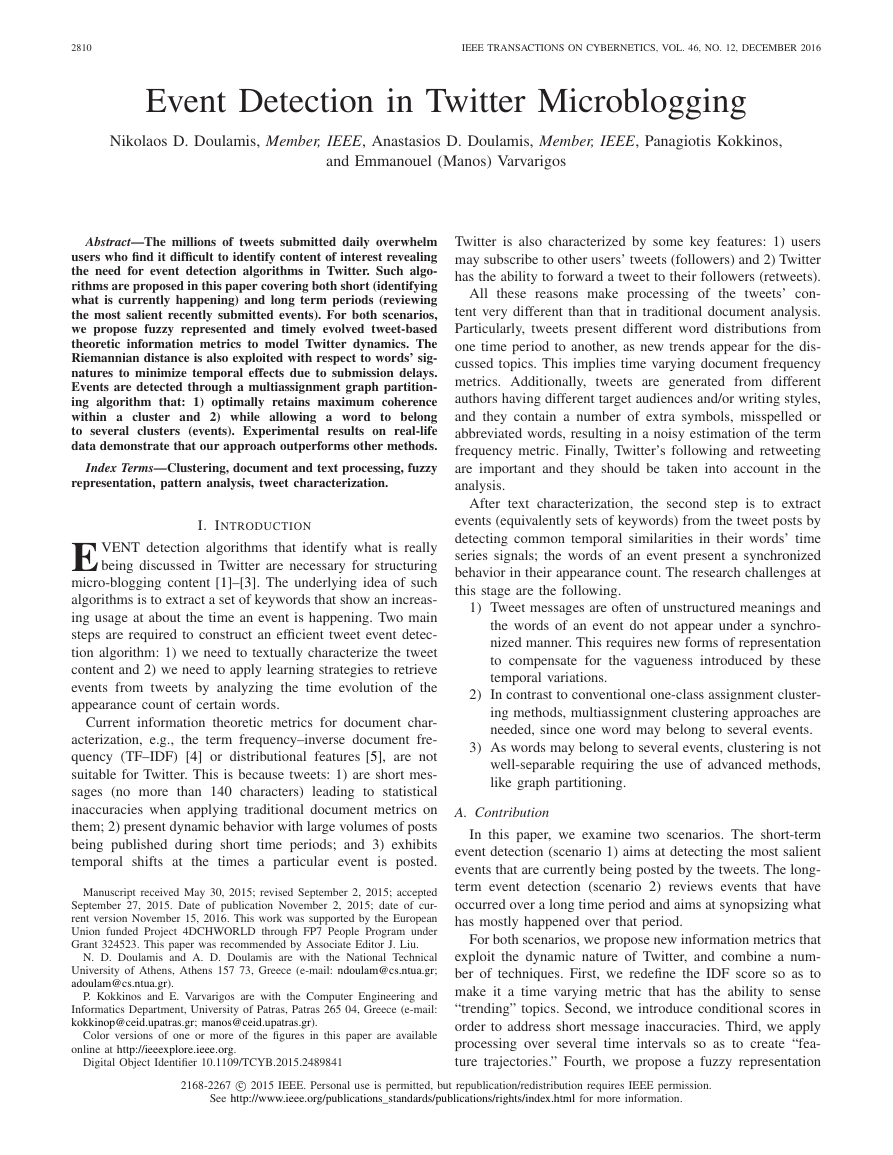
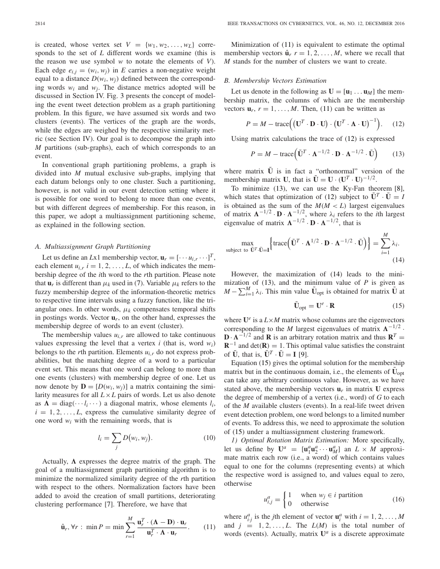
Fig. 1. Operation of the proposed fuzzy representation.
3) Weighted Conditional Word Tweet Frequency–Inverse
Trend Weighted Conditional Word Tweet Frequency: The third
metric, ϑ3(k, w), considers Twitter specific parameters, such as
the number of followers and retweets. The number of follow-
ers indicates authors’ credibility. The number of retweets is
a metric for ranking the importance of the textual content. In
particular, we denote by fm(k), m = 1, . . . , N(k), the num-
ber of followers for the mth tweet at time k, and as rm(k)
the number of retweets. Then, p f
m=1 fm(k)
m=1 rm(k) are their normalized values.
and pr
m
Then
m(k) = fm(k)/
(k) = rm(k)/
N(k)
N(k)
=
N(k)
m=1 p f
m(k) · pr
m=1 p f
m
N(k)
× log
p
j=1
(k) · im(w, k)
m(k) · pr
p
j=1
N(k−j)
m=1 p f
m
N(k−j)
(k)
m=1 p f
m(k − j) · pr
m
m(k − j) · pr
m
(k − j)
(k − j) · im(w, k − j)
(5)
where im(w, k) is an indicator function that equals one if the
mth tweet contains the word w, and zero otherwise.
C. Fuzzy Tweet-Based Representation
We form a time series signal, denoted as xw(k), that contains
the tweet-based information theoretic metrics of (3)–(5) over
a time period of time intervals
xw(k) = [ϑ (k, w)ϑ (k − 1, w)··· ]T .
(6)
In (6), variable ϑ (k, w) refers to one of the three metrics
defined in (3)–(5). Each element ϑ (k, w) of the time series
signal xw(k) expresses the degree of importance of word w at
the kth time interval and in a nonfuzzy representation is calcu-
lated independently of each other. However, in our proposed
fuzzy representation, metric ϑ (k, w) for the kth interval is dif-
fused over K previous intervals but with a different degree of
membership for each interval
ϑf (k, w) = K−1
i=0
ϑ (k − i, w)∗μk(k − i)
(7)
where subscript
f denotes the fuzzy representation of the
respective metric and μk(k−i) is the fuzzy membership degree
for the (k−i)th time interval. The μk takes values in the range
[0, 1]. Usually triangular functions are used to obtain values
of μk but any other fuzzy function can be also adopted. Values
of μk near unity (zero) indicate high (low) degree of member-
ship of the metric. Other types of diffusion methods can also
�
DOULAMIS et al.: EVENT DETECTION IN TWITTER MICROBLOGGING
2813
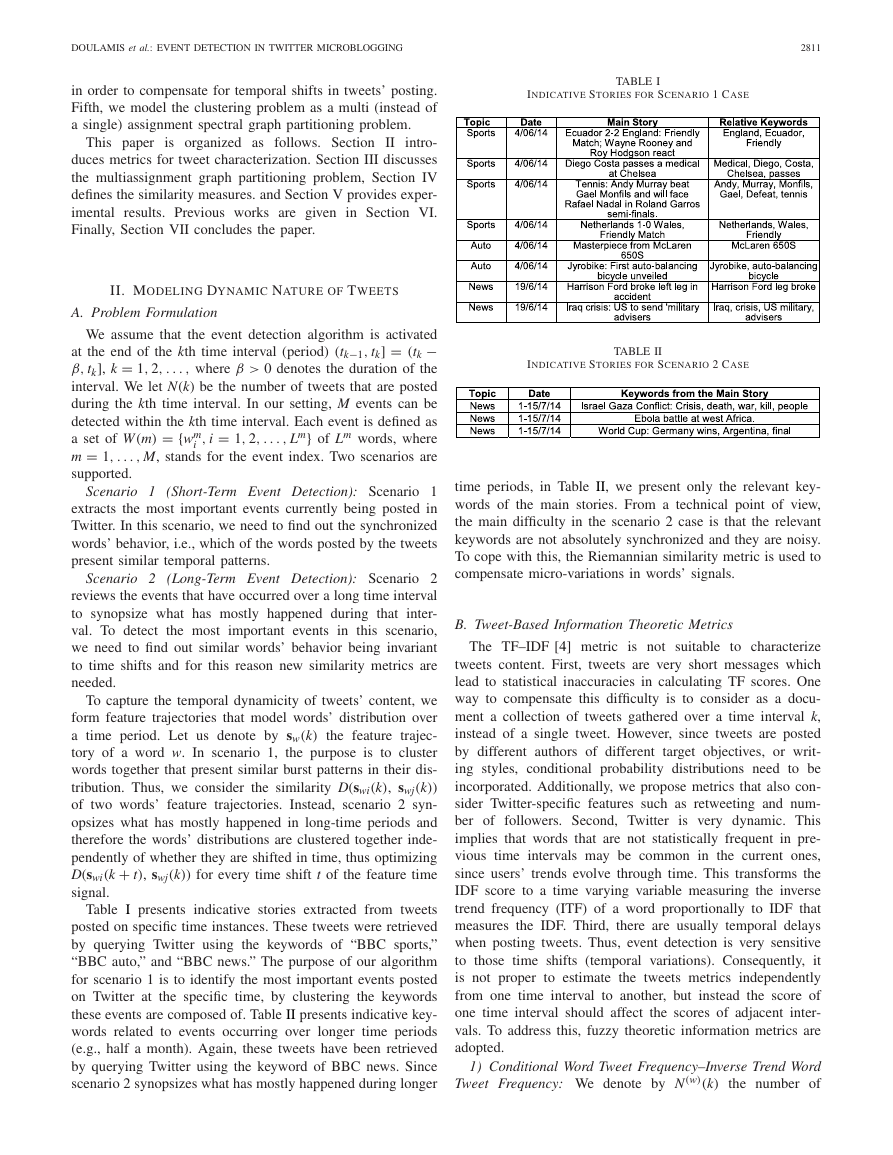
Fig. 2.
(a) Word distribution over ten time intervals. (b) Time series
of the three proposed metrics. The curves with “+” corresponds to fuzzy
representations. The values have been normalized in [0, 1].
be adopted, such as trapezoid, Gaussian, generalized bell, sig-
moid, etc. [6]. Fig. 1 illustrates a graphical representation of
the proposed fuzzy model. Each value ϑ (k, w) is weighed by
membership μk() and the respective product is diffused over
K time intervals. Then, the fuzzy time series signal is
xf ,w(k) =
ϑf (k, w)ϑf (k − 1, w)··· T .
(8)
D. Scale-Time Modeling
To further compensate for the sensitivity of the tweets to
time shifts (temporal variations), we apply the discrete wavelet
transform (DWT) on the signal of (8). The reason we chose
the DWT instead of discrete Fourier transformation (DFT) is
that, unlike the sine/cosine functions used in DFT, which are
localized in frequency but extend infinitely in time, wavelets
are localized both in time and in frequency domain. In partic-
ular, let us denote by sw(k) the wavelet transformed signal of
xf ,w(k), sw(k) ≡ ψ (xf ,w(k)), where ψ (·) refers to the discrete
wavelet operator. Then
w
w
(k)···T
(k)···T ≡ ··· s(i)
sw(k) = ··· c(i,j)
where we denote by c(i,j)
w (k) the jth coefficient of signal sw(k)
at the ith scale and by s(i)
w (k) the ith element of the transformed
wavelet version of signal sw(k) derived by simply renumbering
the wavelet coefficients c(i,j)
w (k). In our approach, we keep the
q wavelet coefficients, preferring the ones derived from the
low pass scale.
(9)
E. Discussion on Example
To better understand the metrics defined above, we consider
a simple synthetic example. Assume we are given N(k) = 10
tweets over ten time intervals, k = 1, . . . , 10. We also
assume eight words per tweet. Then, we construct three time
series xw(k), each for the three metrics ϑ{1,2,3}(k, w). The
tweets are assumed to be organized into three groups. The
first three tweets (1–3) are assumed to have the majority of
followers (most significant tweets), the second group (4–6) is
of medium importance, while the third group (7–10) is of the
lowest importance. We assume 1000 followers for the first
group, 100 followers for the second group, and ten followers
for the third group.
We visualize the appearances of a specific word w over the
ten time intervals as in Fig. 2(a). A white block indicates that
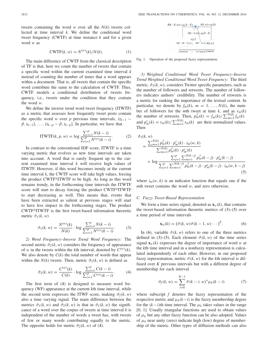
Fig. 3.
problem through graph partitioning.
Schematic depicting the modeling of the event tweet detection
word w appears in the respective tweet. At the first time inter-
val, word w is posted only by one unimportant user. At the
second time interval, two out of the three most important users
tweet word w. At following time intervals, all the important
users followed by the users of intermediate importance sub-
mit word w. Finally, at the last time intervals, the unimportant
users submit the word in their tweets. The meaning of the
example of Fig. 2(a) is that word w initially appears in one
tweet as a noise. Then at the second time interval word w
becomes trendy and therefore starts to be posted by the most
important users, that is, users with many followers. At sub-
sequent time intervals (from the 6th and on), the word w is
not posted by the important users but instead it is propagated
through the tweets of users of medium and low importance.
Fig. 2(b) depicts the time series of the three metrics for
this specific word over the ten different time intervals. We
−6 for
have assumed an initial probability of appearance of 10
word w, i.e., w rarely appears in the previous time intervals.
This initial probability is used for the calculation of ITF score
for the first time interval. For the remaining nine intervals,
ITF term is updated according to the conditional frequency
score computed at a previous time interval [see the first terms
of (3)–(5)]. The values of ϑ (k, w) have been normalized to fit
the range of [0, 1] for better comparisons. As is observed from
Fig. 2(b), the third metric ϑ3(k, w) (5) presents the highest dis-
crimination regarding modeling of w. In particular, ϑ3(k, w)
takes high values only at the time intervals where the impor-
tant users post the word. In contrast, metrics ϑ1(k, w) and
ϑ2(k, w) spread the word’s significance across all intervals
since they handle all tweets equally. Metric ϑ2(k, w) yields
the lowest discrimination accuracy. This is mainly because in
ϑ{1,3}(k, w), a tweet fully contributes to the overall measure
if it contains the specific word (0 or 1 contribution), while in
ϑ2(k, w) a tweet contributes proportionally to the number of
words within this tweet. In Fig. 2(b), we have also depicted
with the “+” mark the fuzzy representations of the respec-
tive metrics. We observe that the fuzzy mapping improves the
discriminatory performance.
III. EVENT DETECTION AS MULTIASSIGNMENT
GRAPH PARTITIONING PROBLEM
Following the analysis of Section II, each word is repre-
sented as a time series signal sw(k). Then, our goal is to
create events consisting of a set of L words by examining
the similarity between the word’s distributions. The value of
L is proportional to the number of the most frequent words
(see Section V-A3). Toward this end, a graph G = {V, E}
�
2814
IEEE TRANSACTIONS ON CYBERNETICS, VOL. 46, NO. 12, DECEMBER 2016
Minimization of (11) is equivalent to estimate the optimal
membership vectors ˆur r = 1, 2, . . . , M, where we recall that
M stands for the number of clusters we want to create.
is created, whose vertex set V = {w1, w2, . . . , wL} corre-
sponds to the set of L different words we examine (this is
the reason we use symbol w to notate the elements of V).
Each edge ei,j = (wi, wj) in E carries a non-negative weight
equal to a distance D(wi, wj) defined between the correspond-
ing words wi and wj. The distance metrics adopted will be
discussed in Section IV. Fig. 3 presents the concept of model-
ing the event tweet detection problem as a graph partitioning
problem. In this figure, we have assumed six words and two
clusters (events). The vertices of the graph are the words,
while the edges are weighed by the respective similarity met-
ric (see Section IV). Our goal is to decompose the graph into
M partitions (sub-graphs), each of which corresponds to an
event.
In conventional graph partitioning problems, a graph is
divided into M mutual exclusive sub-graphs, implying that
each datum belongs only to one cluster. Such a partitioning,
however, is not valid in our event detection setting where it
is possible for one word to belong to more than one events,
but with different degrees of membership. For this reason, in
this paper, we adopt a multiassignment partitioning scheme,
as explained in the following section.
A. Multiassignment Graph Partitioning
Let us define an Lx1 membership vector, ur = [··· ui,r ···]T,
each element ui,r i = 1, 2, . . . , L, of which indicates the mem-
bership degree of the ith word to the rth partition. Please note
that ur is different than μk used in (7). Variable μk refers to the
fuzzy membership degree of the information-theoretic metrics
to respective time intervals using a fuzzy function, like the tri-
angular ones. In other words, μk compensates temporal shifts
in postings words. Vector ur, on the other hand, expresses the
membership degree of words to an event (cluster).
The membership values ui,r are allowed to take continuous
values expressing the level that a vertex i (that is, word wi)
belongs to the rth partition. Elements ui,r do not express prob-
abilities, but the matching degree of a word to a particular
event set. This means that one word can belong to more than
one events (clusters) with membership degree of one. Let us
now denote by D = [D(wi, wj)] a matrix containing the simi-
larity measures for all L×L pairs of words. Let us also denote
as � = diag(··· li ··· ) a diagonal matrix, whose elements li,
i = 1, 2, . . . , L, express the cumulative similarity degree of
one word wi with the remaining words, that is
li =
D
.
wi, wj
j
(10)
Actually, � expresses the degree matrix of the graph. The
goal of a multiassignment graph partitioning algorithm is to
minimize the normalized similarity degree of the rth partition
with respect to the others. Normalization factors have been
added to avoid the creation of small partitions, deteriorating
clustering performance [7]. Therefore, we have that
· (� − D) · ur
uT
r
ˆur,∀r : min P = min
· � · ur
(11)
uT
r
.
M
r=1
(12)
(13)
B. Membership Vectors Estimation
Let us denote in the following as U = [u1 . . . uM] the mem-
bership matrix, the columns of which are the membership
vectors ur, r = 1, . . . , M. Then, (11) can be written as
P = M − trace
UT · D · U
·
UT · � · U
−1
.
Using matrix calculations the trace of (12) is expressed
P = M − trace
˜UT · �−1/2 · D · �−1/2 · ˜U
To minimize (13), we can use the Ky-Fan theorem [8],
where matrix ˜U is in fact a “orthonormal” version of the
membership matrix U, that is ˜U = U · (UT · U)−1/2.
which states that optimization of (12) subject to ˜UT · ˜U = I
is obtained as the sum of the M(M < L) largest eigenvalues
of matrix �−1/2 · D · �−1/2, where λi refers to the ith largest
eigenvalue of matrix �−1/2 · D · �−1/2, that is
˜UT · �1/2 · D · �−1/2 · ˜U
trace
max
λi.
subject to ˜UT· ˜U=I
= M
i=1
(14)
the maximization of (14) leads to the mini-
However,
mization of (13), and the minimum value of P is given as
M −
λi. This min value ˜Uopt is obtained for matrix ˜U at
M
i=1
˜Uopt = Ue · R
Equation (15) gives the optimal solution for the membership
(15)
where Ue is a L×M matrix whose columns are the eigenvectors
corresponding to the M largest eigenvalues of matrix �−1/2 ·
D· �−1/2 and R is an arbitrary rotation matrix and thus RT =
−1 and det(R) = 1. This optimal value satisfies the constraint
R
of ˜U, that is, ˜UT · ˜U = I [9].
matrix but in the continuous domain, i.e., the elements of ˜Uopt
can take any arbitrary continuous value. However, as we have
stated above, the membership vectors ur in matrix U express
the degree of membership of a vertex (i.e., word) of G to each
of the M available clusters (events). In a real-life tweet driven
event detection problem, one word belongs to a limited number
of events. To address this, we need to approximate the solution
of (15) under a multiassignment clustering framework.
1) Optimal Rotation Matrix Estimation: More specifically,
let us define by Ua = [ua
1ua
2
mate matrix each row (i.e., a word) of which contains values
equal to one for the columns (representing events) at which
the respective word is assigned to, and values equal to zero,
otherwise
M] an L × M approxi-
··· ua
=
ua
i,j
1 when wj ∈ i partition
0
otherwise
(16)
i·j is the jth element of vector ua
i with i = 1, 2, . . . , M
where ua
and j = 1, 2, . . . , L. The L(M) is the total number of
words (events). Actually, matrix Ua is a discrete approximate
�
DOULAMIS et al.: EVENT DETECTION IN TWITTER MICROBLOGGING
2815
solution. In contrast to conventional one-cluster assignment
problems, a row of Ua may have more than one unit elements.
In this paper, we propose an iterative methodology that
recursively estimates an optimal rotation matrix ˆR in a way
to update the continuous solution Ue · R to be closest to the
discrete one. In particular, matrix ˆR is estimated through the
min ˆR = arg min
following constrained minimization problem [10]:
subject to RT = R
Ua − Ue · R
−1.
(17)
The solution of (17) can be expressed as an singular value
decomposition problem
ˆR = � · �T and UaT · Ue = � · � · �T
(18)
where (�, �, �) is the singular value decomposition of
UaT · Ue with �T · � = I and �T · � = I.
C. Multiassignment Clustering Approximation
A simple rounding mechanism is to set the maximum value
of each row of the continuous solution equal to 1 and the
other to 0. This approach has the drawback that it is valid
only for a single-assignment method (which is not our case),
and its performance is not satisfactory when there is no clear
dominant maximum value. In this paper, we adopt as rounding
process a novel method, appropriate for the multiassignment
clustering problem. Initially, the algorithm starts assuming
a hard one-class assignment, and then the problem is relaxed.
In particular, we treat the L rows of the continuous solution
as an M-dimensional feature vector and then we apply the
k-means algorithm to assign the L rows (words) to one of the
M available clusters (events). The main concept is to assign
each word to only one cluster that fits best. Using this step
we create M mutual exclusive sets (that correspond to the M
events) ˜W(m), m = 1, . . . , M. Let us denote as umin
m the min-
imum membership value over all words wi ∈ ˜W(m) for the
event ˜W(m)
= min ui,m ∀wi ∈ W(m)
umin
m
(19)
where ui,m is the membership value of the ith word to the mth
event. Using (19), we are able to extend sets ˜W(m) to fit the
multiassignment clustering problem as
W(m) = ˜W(m) ∪
wi : ui,m ≥ umin
m
.
(20)
a better discrete approximation solution. We then discretize
˜Uopt(n) to get Ua(n) as above. Then, using Ua(n) and Ue, we
can derive the new optimal matrix ˆR(n + 1) at the (n + 1)th
iteration by singularly decomposing the matrices UaT (n) · Ue.
E. Estimation of Number of Clusters
As shown in [11], in an ideal case of clean datasets, the
highest magnitude eigenvalue of �−1/2 · D · �−1/2 will be
a repeated eigenvalue of magnitude equal to 1 and multi-
plicity equal to M. Thus, one could estimate M by counting
the number of eigenvalues that are equal to 1. However, if
the clusters are not clearly separated, the magnitudes of the
highest eigenvalues start to deviate from 1, making such a cri-
terion unreliable [12]. An alternative approach is to search for
a drop in the magnitude of the ordered eigenvalues [13]. Since
the eigenvalues depend on the structure of the clusters, no
assumptions can be made on their values, implying that the
eigen-gap can be either small or large [12]. To overcome this
difficulty, [12] introduces a cost function J that relates to the
degree of separability of the clusters, and the optimal number
of clusters is derived as the one that optimizes this cost func-
tion. However, the analysis in [12] assumes a single-cluster
assignment problem, where each sample is assigned to one
cluster. Since, in our case, we have a multiassignment prob-
lem at hand, we need to modify the cost function of [12] to
fit our constraints. In order to do so, recall that ˜Uopt is an
L × M matrix obtained after rotating the eigenvector matrix
Ue (15). Then, if we denote by Ui,j the (i, j) element of ˜Uopt
and let Umax = maxj Ui,j, the optimal number of clusters Mopt
is given as the argument that minimizes the cost function J
Mopt = arg min
M
J = 1
L · ˜M
L
i=1
M
j=1
U2
i,j
U2
max
(21)
where ˜M is the average number of clusters to which a sample
can belong to. Equation (21) means that samples that clearly
belong to a cluster contribute with one to the cost function J,
instead of the samples that are far away from a cluster.
Variable ˜M is estimated by sorting the values of U2
max
in a descending order and then computing the differences
dj = U2
max between two adjacent values, for
j = 1, . . . , M − 1. We also estimate the cumulative values of
these differences. Variable ˜M is computed at the index where
−U2
i,j+1
/U2
/U2
/U2
max
i,j
i,j
Equation (20) means that we append to the initially esti-
mated sets ˜W(m) additional words whose membership values
to this particular event is greater than or equal to umin
m , even
though these words have been assigned to other events.
a drop of the cumulative values below a threshold (e.g., 0.4
in our case) is noticed. We calculate J for different number
of clusters (starting from a minimum value of 2 up to a max-
imum one) and select as the best number of clusters the one
that minimizes J.
D. Dynamically Updating Rotation Matrix
The aforementioned process describes how we can obtain
from the continuous an approximate discrete solution. In this
section, we describe an iterative methodology for updating
the rotation matrix R of (17) to yield a new solution that can
provide a better discrete approximation.
We denote by ˆR(n) the optimal rotation matrix at the nth
iteration of the algorithm. Using matrix ˆR(n), we estimate
a new continuous solution ˜Uopt(n) = Ue· ˆR(n) that can provide
IV. SIMILARITY MEASURES
In this section, we define the similarity metrics among
the words’ time series signals. In particular, we use the
cross-correlation and the Riemannian distance as the simi-
larity metric for scenarios 1 and 2. An essential difference
between the two is that cross-correlation expresses the simi-
larity degree of two signals (takes value one when we have
absolute matching), while Riemannian metric is a distance
�
2816
IEEE TRANSACTIONS ON CYBERNETICS, VOL. 46, NO. 12, DECEMBER 2016
(inverse function of the similarity) that takes value zero in
the matching case. For this reason, in our case, we linearly
normalize the Riemannian metric so that its maximum value
is set to 0 (high dissimilarity) and its minimum is set 1 (high
similarity).
A. Cross-Correlation as for Similarity for Scenario 1
The main limitation of
commonly used
Euclidean distance is that it is sensitive to scaling and/or
translation [14], [15]. For this reason, the normalized cross-
correlation Dcc is adopted in this paper for the scenario 1 case
the most
Dcc(wi, wj) =
sT
wi
· swj
sT
wj
sT
wi
· swi
.
· swj
(22)
B. Riemannian Metric as for Similarity for Scenario 2
The normalized cross-correlation metric is still an “averag-
ing operator.” For instance, using the cross-correlation crite-
rion, it is quite probable for words’ distributions that exhibit
similar behavior but are shifted in time to yield low cross-
correlation values. To address this difficulty, we introduce the
Riemannian geodesic metric [16].
s(k−l)
s(k−l)
T ·
In Section II-D we constructed a wavelet signal s(k)
w of size q
for a given time interval k and word w (q stands for the number
of wavelet coefficients), and defined an q × q autocovariance
matrix Cw with elements
cw(l) = E
(23)
where E{·} denotes the expectation operator. In (23), we have
not added the conventional row/column indices on matrix ele-
ments cw(l) since these elements in fact depend on k − l
distance due to the autocovariance matrix properties.
The q × q symmetric positive definite matrices (nonsin-
gular covariance matrices) can be formulated as connected
Riemannian manifolds. It has been shown in geodesy science
that the distance between the two arbitrary covariance matrices
A and B is given by the following equation [16]:
− E
− E
s(k)
w
s(k)
w
w
w
DR(A, B) =
n
i=1
ln2 λi(A, B).
(24)
In (24), λi(A, B) refers to the ith generalized eigenvalue of
matrices A and B, i.e., A· x = λ· B· x, while n is the number
of generalized eigenvalues. In our case, matrices A and B
are the autocovariance matrices of two words’ distributions,
that is, A ≡ Cwi and A ≡ Cwj for two arbitrary words wi, wj.
C. Discussion on Example
1) Cross-Correlation and Wavelets: We generate eight dif-
ferent word distributions in a similar way to that used for
generating the two signals used in Fig. 2 and we calcu-
late the three metrics ϑ{1,2,3}(k, w) for each of them. Then,
we compute the cross-correlation distance among the time
series signals of all the eight words, resulting in an 8 × 8
cross-correlation matrix for each of the three adopted metrics
ϑ{1,2,3}(k, w).
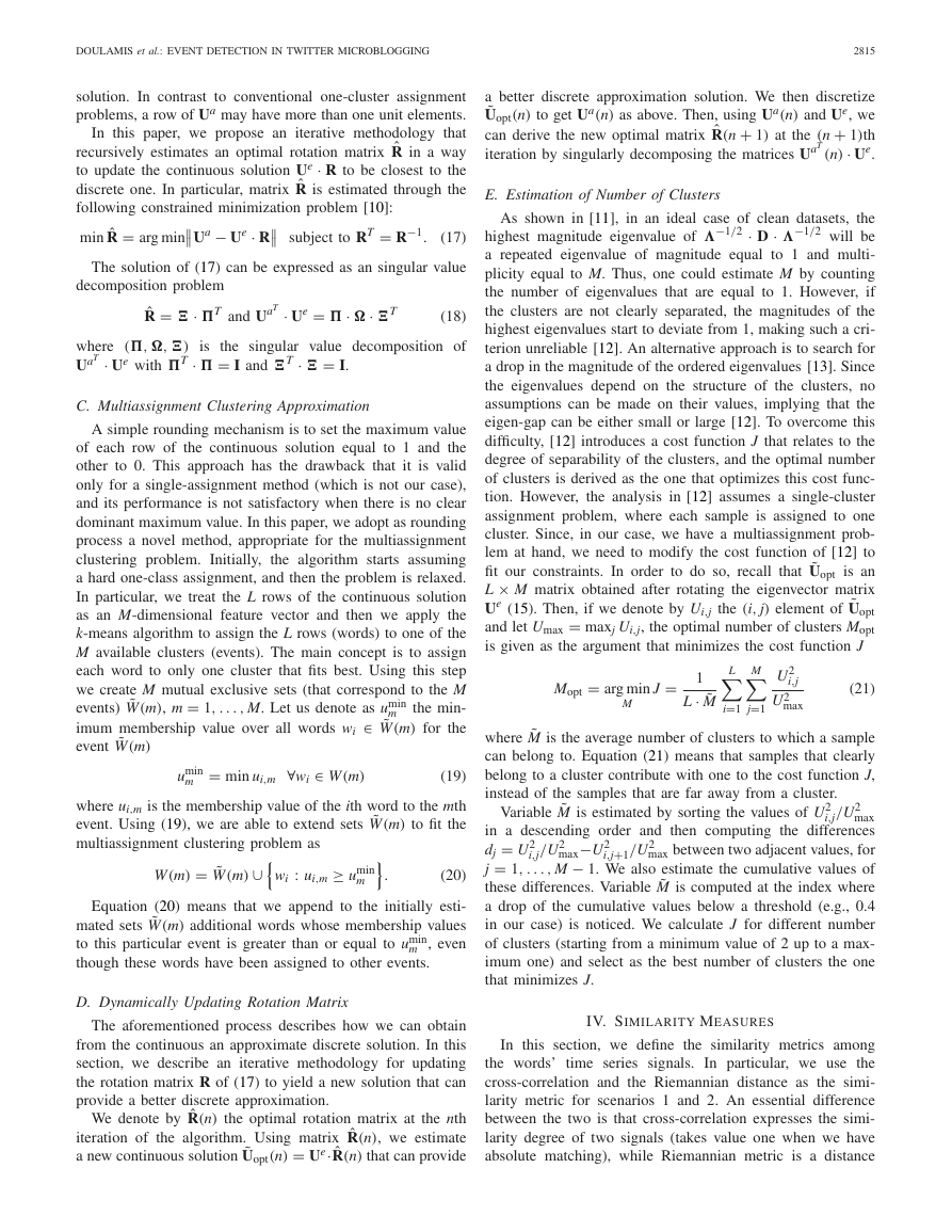
Fig. 4. Discriminatory performance of the cross-correlation distance of one
word against other eight word indices under the fuzzy feature trajectories case;
the similar (dissimilar) word pairs are closer to 1 (0).
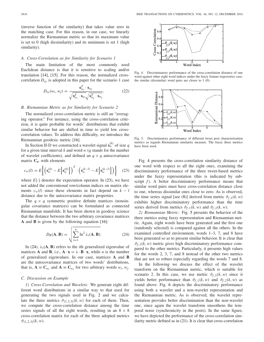
Fig. 5. Discriminatory performance of different tweet post characterization
metrics as regards Riemannian similarity measure. The fuzzy three metrics
have been used.
Fig. 4 presents the cross-correlation similarity distance of
one word with respect to all the eight ones, examining the
discriminatory performance of the three tweet-based metrics
under the fuzzy representation (this is indicated by sub-
script
f ). A better discriminatory performance means that
similar word pairs must have cross-correlation distance close
to one, whereas dissimilar ones close to zero. As is observed,
the time series signal [see (8)] derived from metric ϑf ,3(k, w)
exhibits higher discriminatory performance than the time
series derived from metrics ϑf ,1(k, w) and ϑf ,2(k, w).
2) Riemannian Metric: Fig. 5 presents the behavior of the
three metrics using fuzzy representation and Riemannian met-
ric. Again, eight words have been generated and the first one
(randomly selected) is compared against all the others. In the
examined controlled environment, words 1–3, 7, and 8 have
been generated so as to present similar behavior. It is clear that
ϑf ,3(k, w) metric gives high discriminatory performance com-
pared to the other metrics. Particularly, it presents high values
for the words 2, 3, 7, and 8 instead of the other two metrics
that are not so robust especially regarding the words 7 and 8.
In the following we discuss the effect of the wavelet
transform on the Riemannian metric, which is suitable for
scenario 2. In this case, we use metric ϑf ,3(k, w) since it
yields better performance than ϑf ,1(k, w) and ϑf ,2(k, w) as
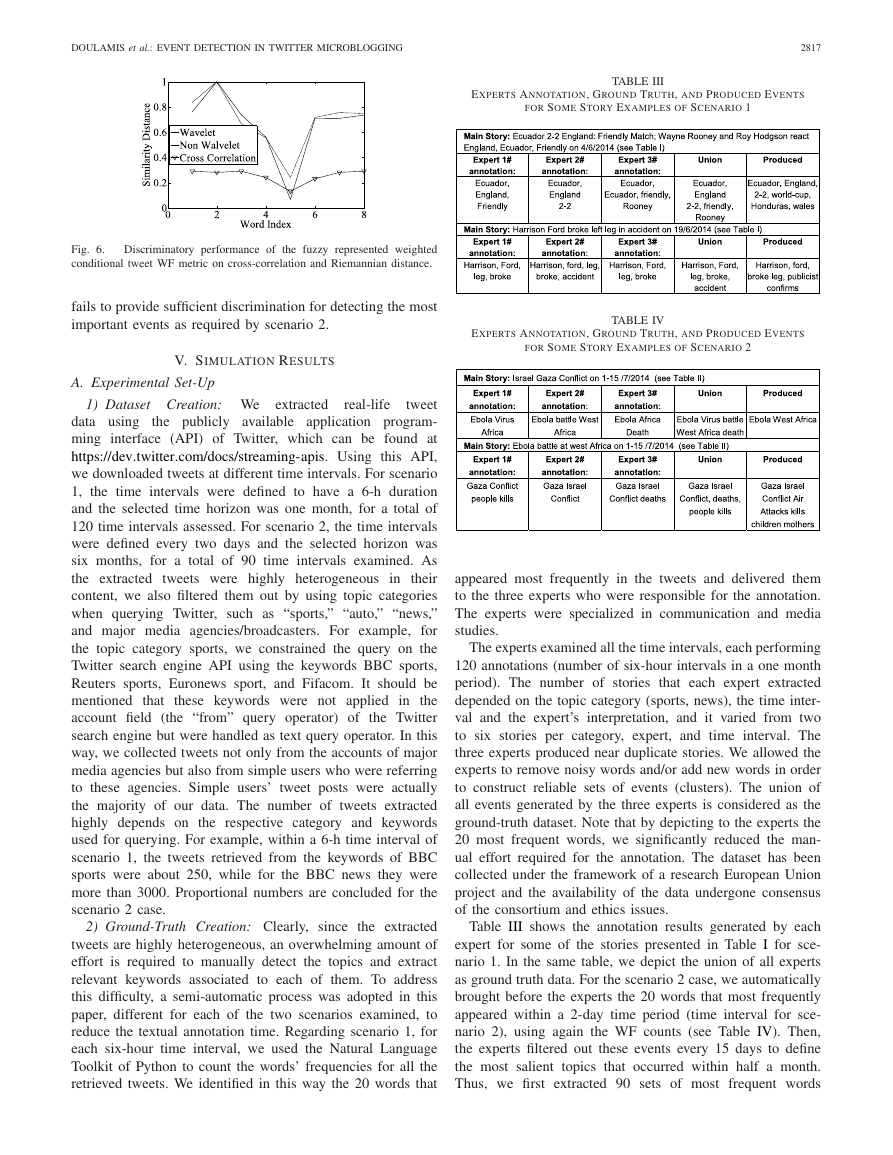
found above. Fig. 6 depicts the discriminatory performance
using both a wavelet and a non-wavelet representation and
the Riemannian metric. As is observed, the wavelet repre-
sentation provides better discrimination than the non-wavelet
one, since again the wavelet transform smoothens the tem-
poral noise (synchronicity in the posts). In the same figure,
we have depicted the performance of the cross-correlation sim-
ilarity metric defined as in (21). It is clear that cross-correlation
�
DOULAMIS et al.: EVENT DETECTION IN TWITTER MICROBLOGGING
2817
EXPERTS ANNOTATION, GROUND TRUTH, AND PRODUCED EVENTS
FOR SOME STORY EXAMPLES OF SCENARIO 1
TABLE III
Fig. 6.
Discriminatory performance of the fuzzy represented weighted
conditional tweet WF metric on cross-correlation and Riemannian distance.
fails to provide sufficient discrimination for detecting the most
important events as required by scenario 2.
V. SIMULATION RESULTS
A. Experimental Set-Up
EXPERTS ANNOTATION, GROUND TRUTH, AND PRODUCED EVENTS
FOR SOME STORY EXAMPLES OF SCENARIO 2
TABLE IV
extracted
real-life
1) Dataset Creation: We
tweet
data using the publicly available application program-
ming interface (API) of Twitter, which can be found at
https://dev.twitter.com/docs/streaming-apis. Using this API,
we downloaded tweets at different time intervals. For scenario
1, the time intervals were defined to have a 6-h duration
and the selected time horizon was one month, for a total of
120 time intervals assessed. For scenario 2, the time intervals
were defined every two days and the selected horizon was
six months, for a total of 90 time intervals examined. As
the extracted tweets were highly heterogeneous in their
content, we also filtered them out by using topic categories
when querying Twitter, such as “sports,” “auto,” “news,”
and major media agencies/broadcasters. For example, for
the topic category sports, we constrained the query on the
Twitter search engine API using the keywords BBC sports,
Reuters sports, Euronews sport, and Fifacom. It should be
mentioned that
these keywords were not applied in the
account field (the “from” query operator) of the Twitter
search engine but were handled as text query operator. In this
way, we collected tweets not only from the accounts of major
media agencies but also from simple users who were referring
to these agencies. Simple users’ tweet posts were actually
the majority of our data. The number of tweets extracted
highly depends on the respective category and keywords
used for querying. For example, within a 6-h time interval of
scenario 1, the tweets retrieved from the keywords of BBC
sports were about 250, while for the BBC news they were
more than 3000. Proportional numbers are concluded for the
scenario 2 case.
2) Ground-Truth Creation: Clearly, since the extracted
tweets are highly heterogeneous, an overwhelming amount of
effort is required to manually detect the topics and extract
relevant keywords associated to each of them. To address
this difficulty, a semi-automatic process was adopted in this
paper, different for each of the two scenarios examined, to
reduce the textual annotation time. Regarding scenario 1, for
each six-hour time interval, we used the Natural Language
Toolkit of Python to count the words’ frequencies for all the
retrieved tweets. We identified in this way the 20 words that
appeared most frequently in the tweets and delivered them
to the three experts who were responsible for the annotation.
The experts were specialized in communication and media
studies.
The experts examined all the time intervals, each performing
120 annotations (number of six-hour intervals in a one month
period). The number of stories that each expert extracted
depended on the topic category (sports, news), the time inter-
val and the expert’s interpretation, and it varied from two
to six stories per category, expert, and time interval. The
three experts produced near duplicate stories. We allowed the
experts to remove noisy words and/or add new words in order
to construct reliable sets of events (clusters). The union of
all events generated by the three experts is considered as the
ground-truth dataset. Note that by depicting to the experts the
20 most frequent words, we significantly reduced the man-
ual effort required for the annotation. The dataset has been
collected under the framework of a research European Union
project and the availability of the data undergone consensus
of the consortium and ethics issues.
Table III shows the annotation results generated by each
expert for some of the stories presented in Table I for sce-
nario 1. In the same table, we depict the union of all experts
as ground truth data. For the scenario 2 case, we automatically
brought before the experts the 20 words that most frequently
appeared within a 2-day time period (time interval for sce-
nario 2), using again the WF counts (see Table IV). Then,
the experts filtered out these events every 15 days to define
the most salient topics that occurred within half a month.
Thus, we first extracted 90 sets of most frequent words
�


 2023年江西萍乡中考道德与法治真题及答案.doc
 2012年重庆南川中考生物真题及答案.doc
 2013年江西师范大学地理学综合及文艺理论基础考研真题.doc
 2020年四川甘孜小升初语文真题及答案I卷.doc
 2020年注册岩土工程师专业基础考试真题及答案.doc
 2023-2024学年福建省厦门市九年级上学期数学月考试题及答案.doc
 2021-2022学年辽宁省沈阳市大东区九年级上学期语文期末试题及答案.doc
 2022-2023学年北京东城区初三第一学期物理期末试卷及答案.doc
 2018上半年江西教师资格初中地理学科知识与教学能力真题及答案.doc
 2012年河北国家公务员申论考试真题及答案-省级.doc
 2020-2021学年江苏省扬州市江都区邵樊片九年级上学期数学第一次质量检测试题及答案.doc
 2022下半年黑龙江教师资格证中学综合素质真题及答案.doc