Cascade Object Detection with Deformable Part Models_CVPR2010.pdf

发布时间：2022-06-14 发布人：admin 分类：说明书资料大小：0.61M 资料格式：pdf 举报版权申诉

0ed9c82f-0621-46aa-8e6a-cc9143f238a4.pdf-第1页.png

第1页 / 共8页

0ed9c82f-0621-46aa-8e6a-cc9143f238a4.pdf-第2页.png

第2页 / 共8页

0ed9c82f-0621-46aa-8e6a-cc9143f238a4.pdf-第3页.png

第3页 / 共8页

0ed9c82f-0621-46aa-8e6a-cc9143f238a4.pdf-第4页.png

第4页 / 共8页

0ed9c82f-0621-46aa-8e6a-cc9143f238a4.pdf-第5页.png

第5页 / 共8页

0ed9c82f-0621-46aa-8e6a-cc9143f238a4.pdf-第6页.png

第6页 / 共8页

0ed9c82f-0621-46aa-8e6a-cc9143f238a4.pdf-第7页.png

第7页 / 共8页

0ed9c82f-0621-46aa-8e6a-cc9143f238a4.pdf-第8页.png

第8页 / 共8页

文本预览

Cascade Object Detection with Deformable Part Models∗ Pedro F. Felzenszwalb University of Chicago pff@cs.uchicago.edu Ross B. Girshick University of Chicago rbg@cs.uchicago.edu David McAllester TTI at Chicago mcallester@ttic.edu Abstract We describe a general method for building cascade clas- siﬁers from part-based deformable models such as pictorial structures. We focus primarily on the case of star-structured models and show how a simple algorithm based on par- tial hypothesis pruning can speed up object detection by more than one order of magnitude without sacriﬁcing de- tection accuracy. In our algorithm, partial hypotheses are pruned with a sequence of thresholds. In analogy to proba- bly approximately correct (PAC) learning, we introduce the notion of probably approximately admissible (PAA) thresh- olds. Such thresholds provide theoretical guarantees on the performance of the cascade method and can be computed from a small sample of positive examples. Finally, we out- line a cascade detection algorithm for a general class of models deﬁned by a grammar formalism. This class in- cludes not only tree-structured pictorial structures but also richer models that can represent each part recursively as a mixture of other parts. 1. Introduction A popular approach for object detection involves reduc- ing the problem to binary classiﬁcation. The simplest and most common example of this approach is the sliding win- dow method. In this method a classiﬁer is applied at all positions, scales, and, in some cases, orientations of an im- age. However, testing all points in the search space with a non-trivial classiﬁer can be very slow. An effective method for addressing this problem involves applying a cascade of simple tests to each hypothesized object location to elimi- nate most of them very quickly [16, 12, 4, 15, 2, 13]. Another line of research, separate from cascade classi- ﬁers, uses part-based deformable models for detection. In this case an object hypothesis speciﬁes a conﬁguration of parts, which leads to a very large (exponential) hypothesis space. There has been signiﬁcant success in algorithmic methods for searching over these large hypothesis spaces, including methods that are “asymptotically optimal” for tree-structured models [9]. However, these methods are still ∗This research has been supported by NSF grant IIS-0746569. 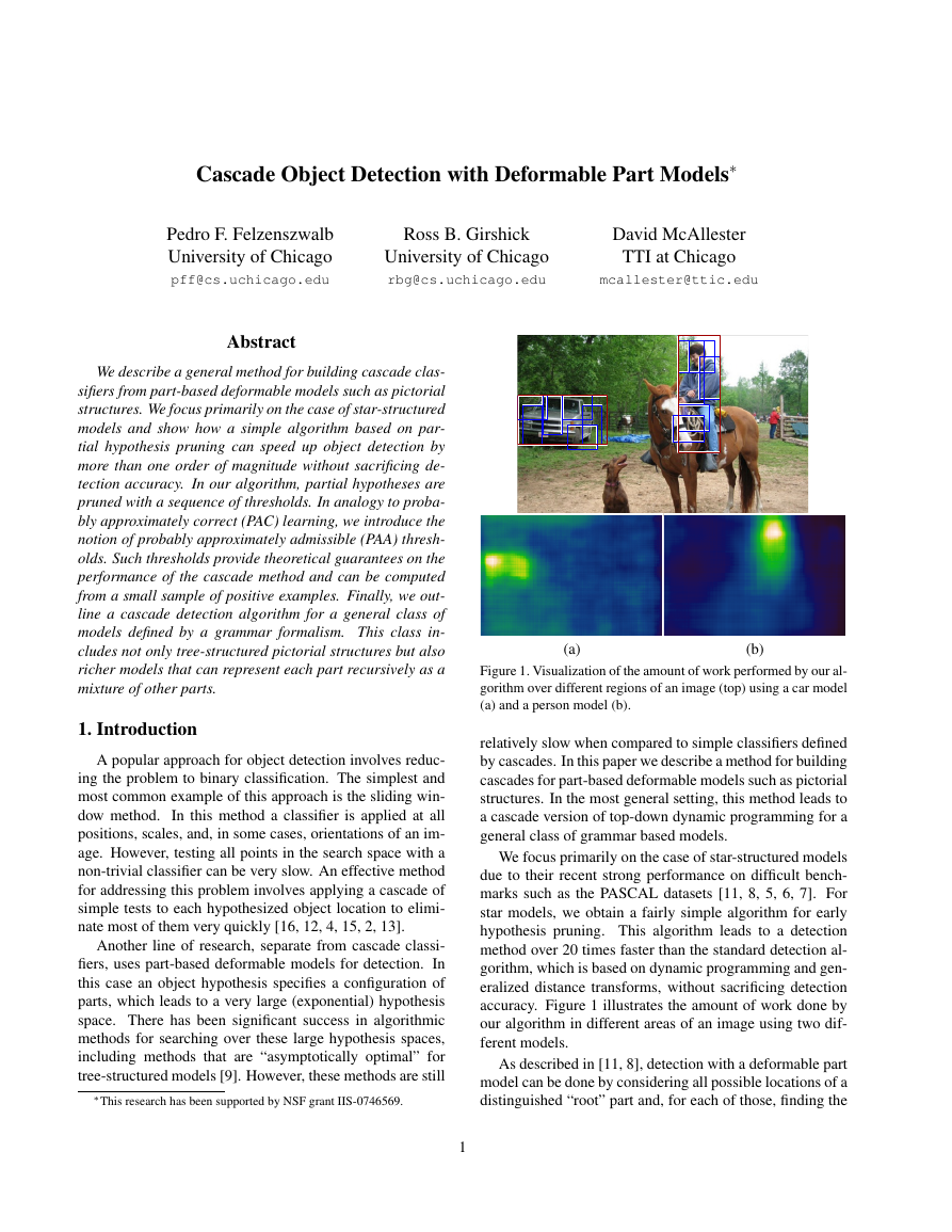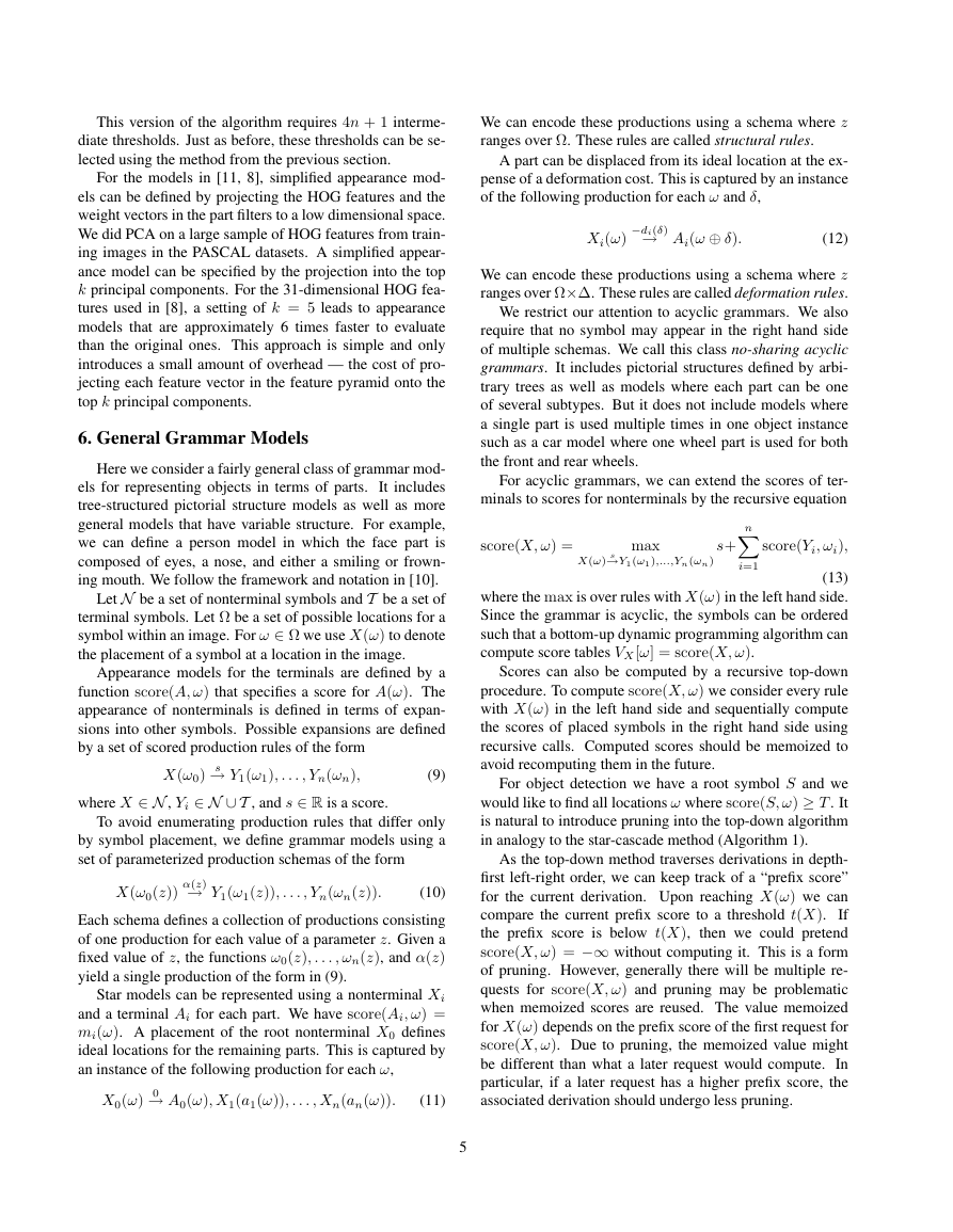(a) (b) Figure 1. Visualization of the amount of work performed by our al- gorithm over different regions of an image (top) using a car model (a) and a person model (b). relatively slow when compared to simple classiﬁers deﬁned by cascades. In this paper we describe a method for building cascades for part-based deformable models such as pictorial structures. In the most general setting, this method leads to a cascade version of top-down dynamic programming for a general class of grammar based models. We focus primarily on the case of star-structured models due to their recent strong performance on difﬁcult bench- marks such as the PASCAL datasets [11, 8, 5, 6, 7]. For star models, we obtain a fairly simple algorithm for early hypothesis pruning. This algorithm leads to a detection method over 20 times faster than the standard detection al- gorithm, which is based on dynamic programming and gen- eralized distance transforms, without sacriﬁcing detection accuracy. Figure 1 illustrates the amount of work done by our algorithm in different areas of an image using two dif- ferent models. As described in [11, 8], detection with a deformable part model can be done by considering all possible locations of a distinguished “root” part and, for each of those, ﬁnding the 1

best conﬁguration of the remaining parts. In this case we need to compute an optimal conﬁguration for each location of the root. These problems are not independent because the possible locations of the remaining parts are shared among different root locations. For tree-structured models one can use dynamic programming to account for this sharing [9]. In practice one is only interested in root locations that lead to high scoring conﬁgurations. The basic idea of our algorithm is to use a hierarchy of models deﬁned by an or- dering of the original model’s parts. For a model with n + 1 parts, including the root, we obtain a sequence of n + 1 models. The i-th model in this sequence is deﬁned by the ﬁrst i parts from the original model. Using this hierarchy, we can prune low scoring hypotheses after looking at the best conﬁguration of a subset of the parts. Hypotheses that score high under a weak model are evaluated further us- ing a richer model. This process is analogous to a classi- cal cascade and is similar to the cascades of [2, 15] in that the score of a weaker model is reused when computing the score of a richer one. However, when using deformable part models individual applications of the cascade are not inde- pendent, so, in analogy to classical dynamic programming, work done evaluating one hypothesis is also reused when evaluating others. Our sequential search for parts is related to [1], where the authors propose a sequential search for semi-local fea- tures that ﬁt a global arrangement. The work in [1] also considered the problem of selecting parameters that lead to fast search with a low false negative rate, by making some assumptions on the form of the distribution of local features and analyzing statistics of training data. We use an alter- native approach (see below) that makes fewer assumptions and relies more heavily on the training data. The time it takes to evaluate a hypothesis for a part-based model is highly dependent on the complexity of the individ- ual part models. Besides simplifying a model by removing some of its parts, we also consider simpliﬁcations that arise from replacing the original part appearance models with simpler ones that are much faster to compute. In this case, for a model with n + 1 parts we get a hierarchy of 2(n + 1) models. The ﬁrst n + 1 models are obtained by sequen- tially adding parts with simpliﬁed appearance models. The second n + 1 models are obtained by sequentially replacing each simpliﬁed appearance model with its full one. Our algorithm prunes partial hypotheses using thresh- olds on their scores. Admissible thresholds would not prune any partial hypothesis that leads to a complete detection scoring above a global threshold. We deﬁne the error of a set of thresholds to be the fraction of full hypotheses scor- ing above the global threshold that are incorrectly pruned. To select pruning thresholds, we introduce the notion of probably approximately admissible (PAA) thresholds. PAA thresholds have a low error with high probability. We show that PAA thresholds can be obtained by looking at statistics of partial hypothesis scores over positive exam- ples. This leads to a simple method for picking safe and effective thresholds. The thresholds are safe because they have low error with high probability. They are effective be- cause they lead to a fast cascade with signiﬁcant pruning. [9] notes that by using dynamic programming and dis- tance transforms the relationships among parts in a tree- structured model can be taken into account “for free.” That is, it takes very little additional time to detect whole object conﬁgurations as opposed to individually detecting parts on their own. Our results push this idea further. In practice we ﬁnd that it is possible to detect whole object conﬁgurations much faster than detecting each individual part. 2. Object Detection with Star Models We start by deﬁning a general framework for object de- tection with star-structured deformable part models that in- cludes the setting in [11, 8]. Let M be a model with a root part v0 and n additional parts v1, . . . , vn. Let Ω be a space of locations for each part within an image. For example, ω ∈ Ω could specify a position and scale. Let mi(ω) be the score for placing vi in location ω. This score depends on the image data, but we assume the image is implicitly deﬁned to simplify notation. For a non-root part, let ai(ω) specify the ideal location for vi as a function of the root location. Let ∆ be a space of displacements, and let ⊕ : Ω × ∆ → Ω be a binary op- eration taking a location and a displacement to a “displaced location.” Let di(δ) specify a deformation cost for a dis- placement of vi from its ideal location relative to the root. An object conﬁguration speciﬁes a location for the root and a displacement for each additional part from its ideal location relative to the root. The score of a conﬁguration is the sum of the scores of the parts at their locations minus deformation costs associated with each displacement. score(ω, δ1, . . . , δn) = n i=1 m0(ω) + mi(ai(ω) ⊕ δi) − di(δi) (1) We can deﬁne an overall score for a root location based on the maximum score of a conﬁguration rooted at that lo- cation. In a star model each part is only attached to the root, so the score can be factored as follows. n scorei(ai(ω)) (mi(η ⊕ δi) − di(δi)) i=1 (2) (3) score(ω) = m0(ω) + scorei(η) = max δi∈∆ Here scorei(η) is the maximum, over displacements of the part from its ideal location, of the part score minus the de- formation cost associated with the displacement. 2

For a ﬁxed global threshold T , any input to Algorithm 1 that correctly computes score(ω) whenever it is above T is called a T -admissible set of thresholds. If given T - admissible thresholds, Algorithm 1 returns exactly the same set of detections as the standard dynamic programming al- gorithm. In the next section we investigate the case of good inadmissible thresholds that produce a cascade with a low error rate but still allow aggressive pruning. The worst-case time of Algorithm 1 is O(n|Ω||∆|) if mi(ω) is taken to cost O(1), which is slower than the stan- dard dynamic programming algorithm with distance trans- forms. However, in practice, for typical models ∆ can be safely made relatively small (c.f . Section 6). Moreover, searching over ∆ is usually no more expensive than eval- uating mi(ω) at a single location, because the spatial extent of a part is of similar size as its range of displacement. The worse-case time of both methods is the same, O(n|Ω||∆|), if we assume evaluating mi(ω) takes O(|∆|) time. 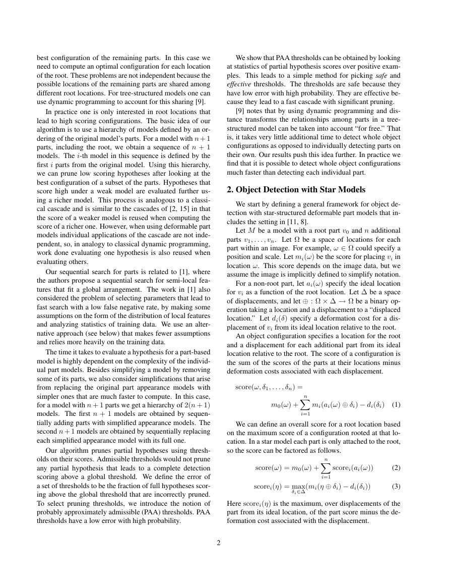n)) and T 1), . . . , (tn, t Data: Thresholds ((t1, t Result: Set of detections D D ← ∅ for ω ∈ Ω do s ← ˜m0(ω) for i = 1 to n do if s < ti then skip ω p ← −∞ for δ ∈ ∆ do if s − di(δ) < t p ← max(p, ˜mi(ai(ω) ⊕ δ) − di(δ)) i then skip δ end s ← s + p end if s ≥ T then D ← D ∪ {ω} For the models in [11, 8], mi(ω) is the response of a ﬁl- ter in a dense feature pyramid, and di(δ) is a (separable) quadratic function of δ. To detect objects [11, 8] look for root locations with an overall score above some threshold, score(ω) ≥ T . A dynamic programming algorithm is used to compute score(ω) for every location ω ∈ Ω. Using the fast distance transforms method from [9] the detection al- gorithm runs in O(n|Ω|) time if we assume that evaluating the appearance model for a part at a speciﬁc location takes O(1) time. In practice, evaluating the appearance models is the bottleneck of the method. 3. Star-Cascade Detection Here we describe a cascade algorithm for star models that uses a sequence of thresholds to prune detections using subsets of parts. Note that we are only interested in root locations where score(ω) ≥ T . By evaluating parts in a sequential order we can avoid evaluating the appearance model for most parts almost everywhere. 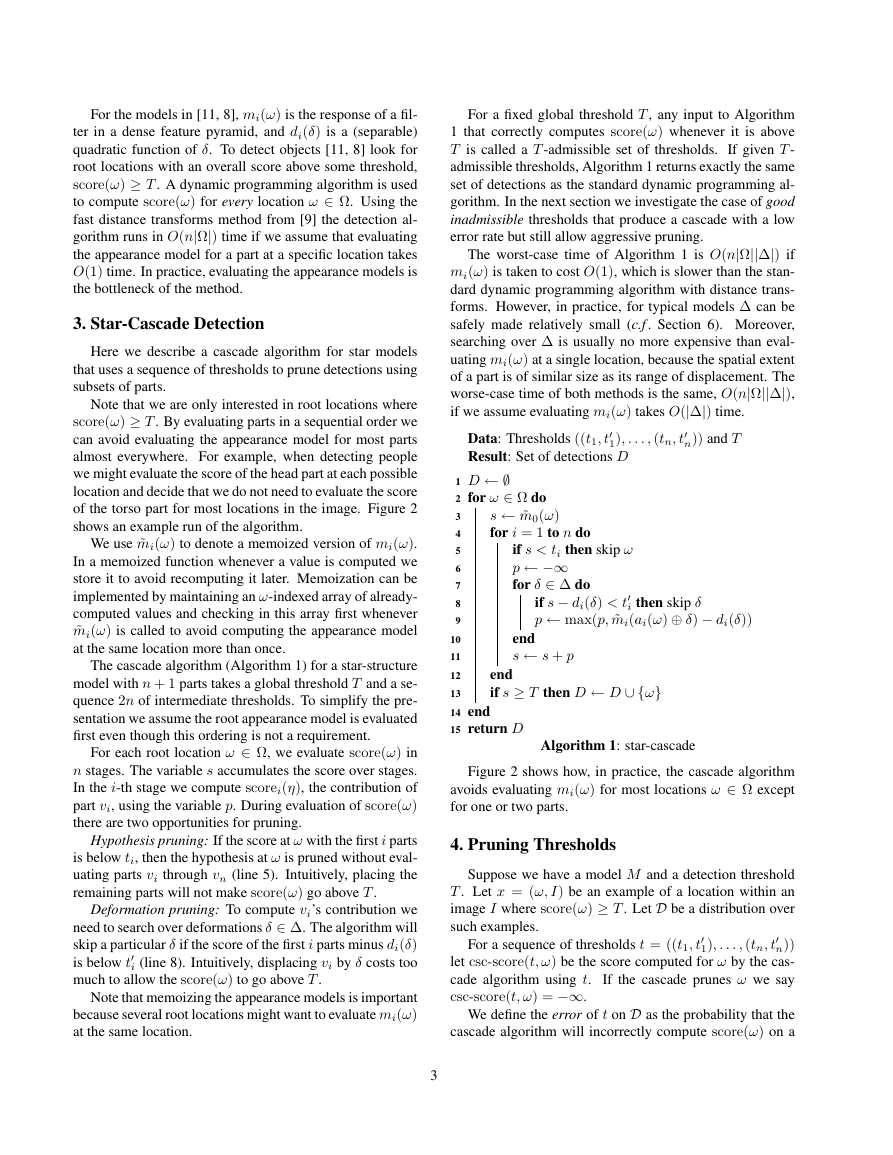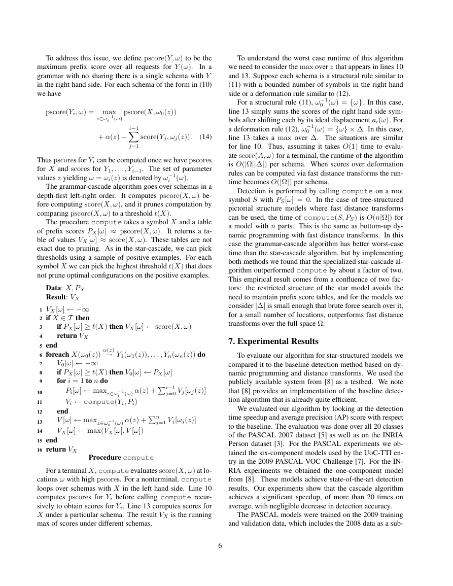For example, when detecting people we might evaluate the score of the head part at each possible location and decide that we do not need to evaluate the score of the torso part for most locations in the image. Figure 2 shows an example run of the algorithm. We use ˜mi(ω) to denote a memoized version of mi(ω). In a memoized function whenever a value is computed we store it to avoid recomputing it later. Memoization can be implemented by maintaining an ω-indexed array of already- computed values and checking in this array ﬁrst whenever ˜mi(ω) is called to avoid computing the appearance model at the same location more than once. The cascade algorithm (Algorithm 1) for a star-structure model with n + 1 parts takes a global threshold T and a se- quence 2n of intermediate thresholds. To simplify the pre- sentation we assume the root appearance model is evaluated ﬁrst even though this ordering is not a requirement. For each root location ω ∈ Ω, we evaluate score(ω) in n stages. The variable s accumulates the score over stages. In the i-th stage we compute scorei(η), the contribution of part vi, using the variable p. During evaluation of score(ω) there are two opportunities for pruning. Hypothesis pruning: If the score at ω with the ﬁrst i parts is below ti, then the hypothesis at ω is pruned without eval- uating parts vi through vn (line 5). Intuitively, placing the remaining parts will not make score(ω) go above T . Deformation pruning: To compute vi’s contribution we need to search over deformations δ ∈ ∆. The algorithm will skip a particular δ if the score of the ﬁrst i parts minus di(δ) is below t i (line 8). Intuitively, displacing vi by δ costs too much to allow the score(ω) to go above T . Note that memoizing the appearance models is important because several root locations might want to evaluate mi(ω) at the same location. 1 2 3 4 5 6 7 8 9 10 11 12 13 14 15 end return D Algorithm 1: star-cascade Figure 2 shows how, in practice, the cascade algorithm avoids evaluating mi(ω) for most locations ω ∈ Ω except for one or two parts. 4. Pruning Thresholds Suppose we have a model M and a detection threshold T . Let x = (ω, I) be an example of a location within an image I where score(ω) ≥ T . Let D be a distribution over such examples. For a sequence of thresholds t = ((t1, t n)) let csc-score(t, ω) be the score computed for ω by the cas- If the cascade prunes ω we say cade algorithm using t. csc-score(t, ω) = −∞. We deﬁne the error of t on D as the probability that the cascade algorithm will incorrectly compute score(ω) on a 1), . . . , (tn, t 3

Figure 2. A sample image with a bicycle detection (left). Each image in the right shows (in white) positions where a particular part appearance model was evaluated at the scale of the bicycle detection. The images are shown in “cascade order” from left to right and top to bottom. The image for the root part, which was evaluated ﬁrst, is not shown because its appearance model is evaluated at all locations. After evaluating the ﬁrst non-root part, nearly all locations were pruned by the cascade. random example from D, error(t) = Px∼D(csc-score(t, ω) = score(ω)). (4) We would like to ﬁnd a sequence of thresholds that has a small error. Note that in practice we are only interested in having a small error on positive examples. In particular we do not care if the cascade incorrectly prunes a negative example that scores above T . Thus we can take D to be a distribution over high-scoring positive examples. Below we show that we can learn a good sequence of thresholds by looking at a small number of examples from D. In analogy to PAC learning [14] we would like to select thresholds that have a small error with high probability. We say a sequence of thresholds t is (, δ) probably ap- proximately admissible (PAA) if the probability that the er- ror of t is greater than is bounded by δ, P (error(t) > ) ≤ δ. (5) Let δ1, . . . , δn be the optimal displacements for the non- root parts of M on an example x = (ω, I). We can deﬁne partial scores that take into account the ﬁrst i parts and the ﬁrst i parts minus the i-th deformation cost, i−1 xi = m0(ω) + i = xi − di(δi). x j=1 mj(aj(ω) + δj) − dj(δj), (6) (7) The star-cascade algorithm will ﬁnd an optimal conﬁgura- tion and score for x if and only if xi ≥ ti and x i for all 1 ≤ i ≤ n. Let X be m independent samples from D. We can select i ≥ t thresholds by picking, ti = min x∈X xi t i = min x∈X x i (8) These are the tightest thresholds that make no mistakes on X. The following theorem shows they also have low error with high probability provided that m is sufﬁciently large. 4 Theorem 1. If we select t according to equation (8) using m ≥ 2n/ ln(2n/δ) samples from D then t is (, δ) proba- bly approximately admissible with respect to D. Proof. By a union bound error(t) ≤ if Px∼D(xi < ti) i) are ≤ /(2n) for all i. Thus error(t) ≤ and Px∼D(x unless for some i all m samples of the xi or x i are above the /(2n)-th percentile of their distribution. The probabil- ity of that event is ≤ 2n(1 − /(2n))m. To bound this by δ we only need m ≥ 2n/ ln(2n/δ) samples. i < t 5. Simpliﬁed Part Appearance Models So far we have considered a cascade for star models that is deﬁned by a hierarchy of n + 1 models. Given a prede- ﬁned part order, the i-th model is formed by adding the i-th part to the (i − 1)-st model. The goal of the cascade is to detect objects while making as few appearance model eval- uations as possible. The star-cascade algorithm achieves this goal by pruning hypotheses using intermediate scores. A complementary approach is to consider a simpliﬁed appearance model for each part, ˆmi(ω), that computes an inexpensive approximation of mi(ω). A hierarchy of 2(n + 1) models can be deﬁned with the ﬁrst n + 1 models constructed as before, but using the sim- pliﬁed appearance models, and the second n + 1 models deﬁned by sequentially removing one of the remaining sim- pliﬁed appearance models ˆmi and replacing it with the orig- inal one mi. With simpliﬁed parts, the star-cascade operates as before for stages 1 through n+1, except that pruning decisions are based on the (memoized) evaluations of the simpliﬁed ap- pearance models ˆmi(ω). During the remaining stages, full appearance models replace simpliﬁed ones. When replacing an appearance model, the algorithm must redo the search over the deformation space because the optimal placement may change. But now we will often prune a hypothesis be- fore evaluating any of the expensive appearance models.

This version of the algorithm requires 4n + 1 interme- diate thresholds. Just as before, these thresholds can be se- lected using the method from the previous section. For the models in [11, 8], simpliﬁed appearance mod- els can be deﬁned by projecting the HOG features and the weight vectors in the part ﬁlters to a low dimensional space. We did PCA on a large sample of HOG features from train- ing images in the PASCAL datasets. A simpliﬁed appear- ance model can be speciﬁed by the projection into the top k principal components. For the 31-dimensional HOG fea- tures used in [8], a setting of k = 5 leads to appearance models that are approximately 6 times faster to evaluate than the original ones. This approach is simple and only introduces a small amount of overhead — the cost of pro- jecting each feature vector in the feature pyramid onto the top k principal components. 6. General Grammar Models Here we consider a fairly general class of grammar mod- els for representing objects in terms of parts. It includes tree-structured pictorial structure models as well as more general models that have variable structure. For example, we can deﬁne a person model in which the face part is composed of eyes, a nose, and either a smiling or frown- ing mouth. We follow the framework and notation in [10]. Let N be a set of nonterminal symbols and T be a set of terminal symbols. Let Ω be a set of possible locations for a symbol within an image. For ω ∈ Ω we use X(ω) to denote the placement of a symbol at a location in the image. Appearance models for the terminals are deﬁned by a function score(A, ω) that speciﬁes a score for A(ω). The appearance of nonterminals is deﬁned in terms of expan- sions into other symbols. Possible expansions are deﬁned by a set of scored production rules of the form X(ω0) s→ Y1(ω1), . . . , Yn(ωn), (9) where X ∈ N , Yi ∈ N ∪T , and s ∈ R is a score. To avoid enumerating production rules that differ only by symbol placement, we deﬁne grammar models using a set of parameterized production schemas of the form X(ω0(z)) α(z)→ Y1(ω1(z)), . . . , Yn(ωn(z)). (10) Each schema deﬁnes a collection of productions consisting of one production for each value of a parameter z. Given a ﬁxed value of z, the functions ω0(z), . . . , ωn(z), and α(z) yield a single production of the form in (9). Star models can be represented using a nonterminal Xi and a terminal Ai for each part. We have score(Ai, ω) = mi(ω). A placement of the root nonterminal X0 deﬁnes ideal locations for the remaining parts. This is captured by an instance of the following production for each ω, X0(ω) 0→ A0(ω), X1(a1(ω)), . . . , Xn(an(ω)). (11) We can encode these productions using a schema where z ranges over Ω. These rules are called structural rules. A part can be displaced from its ideal location at the ex- pense of a deformation cost. This is captured by an instance of the following production for each ω and δ, Xi(ω) −di(δ)→ Ai(ω ⊕ δ). (12) We can encode these productions using a schema where z ranges over Ω×∆. These rules are called deformation rules. We restrict our attention to acyclic grammars. We also require that no symbol may appear in the right hand side of multiple schemas. We call this class no-sharing acyclic grammars. It includes pictorial structures deﬁned by arbi- trary trees as well as models where each part can be one of several subtypes. But it does not include models where a single part is used multiple times in one object instance such as a car model where one wheel part is used for both the front and rear wheels. For acyclic grammars, we can extend the scores of ter- minals to scores for nonterminals by the recursive equation score(X, ω) = max s+ score(Yi, ωi), n i=1 X(ω) s→Y1(ω1),...,Yn(ωn) (13) where the max is over rules with X(ω) in the left hand side. Since the grammar is acyclic, the symbols can be ordered such that a bottom-up dynamic programming algorithm can compute score tables VX[ω] = score(X, ω). Scores can also be computed by a recursive top-down procedure. To compute score(X, ω) we consider every rule with X(ω) in the left hand side and sequentially compute the scores of placed symbols in the right hand side using recursive calls. Computed scores should be memoized to avoid recomputing them in the future. For object detection we have a root symbol S and we would like to ﬁnd all locations ω where score(S, ω) ≥ T . It is natural to introduce pruning into the top-down algorithm in analogy to the star-cascade method (Algorithm 1). As the top-down method traverses derivations in depth- ﬁrst left-right order, we can keep track of a “preﬁx score” for the current derivation. Upon reaching X(ω) we can compare the current preﬁx score to a threshold t(X). If the preﬁx score is below t(X), then we could pretend score(X, ω) = −∞ without computing it. This is a form of pruning. However, generally there will be multiple re- quests for score(X, ω) and pruning may be problematic when memoized scores are reused. The value memoized for X(ω) depends on the preﬁx score of the ﬁrst request for score(X, ω). Due to pruning, the memoized value might be different than what a later request would compute. In particular, if a later request has a higher preﬁx score, the associated derivation should undergo less pruning. 5

To address this issue, we deﬁne pscore(Y, ω) to be the maximum preﬁx score over all requests for Y (ω). In a grammar with no sharing there is a single schema with Y in the right hand side. For each schema of the form in (10) we have pscore(Yi, ω) = max −1 i z∈ω (ω) pscore(X, ω0(z)) i−1 + α(z) + score(Yj, ωj(z)). (14) j=1 i Thus pscores for Yi can be computed once we have pscores for X and scores for Y1, . . . , Yi−1. The set of parameter values z yielding ω = ωi(z) is denoted by ω−1 (ω). The grammar-cascade algorithm goes over schemas in a It computes pscore(X, ω) be- depth-ﬁrst left-right order. fore computing score(X, ω), and it prunes computation by comparing pscore(X, ω) to a threshold t(X). The procedure compute takes a symbol X and a table of preﬁx scores PX[ω] ≈ pscore(X, ω). It returns a ta- ble of values VX[ω] ≈ score(X, ω). These tables are not exact due to pruning. As in the star-cascade, we can pick thresholds using a sample of positive examples. For each symbol X we can pick the highest threshold t(X) that does not prune optimal conﬁgurations on the positive examples. Data: X, PX Result: VX VX[ω] ← −∞ if X ∈ T then if PX[ω] ≥ t(X) then VX[ω] ← score(X, ω) return VX end foreach X(ω0(z)) α(z)→ Y1(ω1(z)), . . . , Yn(ωn(z)) do V0[ω] ← −∞ if PX[ω] ≥ t(X) then V0[ω] ← PX[ω] for i = 1 to n do −1 i (ω) α(z) +i−1 0 (ω) α(z) +n Pi[ω] ← maxz∈ω Vi ← compute(Yi, Pi) end V [ω] ← maxz∈ω VX[ω] ← max(VX[ω], V [ω]) −1 j=0 Vj[ωj(z)] j=1 Vj[ωj(z)] 1 2 3 4 5 6 7 8 9 10 11 12 13 14 15 16 end return VX Procedure compute For a terminal X, compute evaluates score(X, ω) at lo- cations ω with high pscores. For a nonterminal, compute loops over schemas with X in the left hand side. Line 10 computes pscores for Yi before calling compute recur- sively to obtain scores for Yi. Line 13 computes scores for X under a particular schema. The result VX is the running max of scores under different schemas. 6 For a structural rule (11), ω−1 To understand the worst case runtime of this algorithm we need to consider the max over z that appears in lines 10 and 13. Suppose each schema is a structural rule similar to (11) with a bounded number of symbols in the right hand side or a deformation rule similar to (12). 0 (ω) = {ω}. In this case, line 13 simply sums the scores of the right hand side sym- bols after shifting each by its ideal displacement ai(ω). For 0 (ω) = {ω} × ∆. In this case, a deformation rule (12), ω−1 line 13 takes a max over ∆. The situations are similar for line 10. Thus, assuming it takes O(1) time to evalu- ate score(A, ω) for a terminal, the runtime of the algorithm is O(|Ω||∆|) per schema. When scores over deformation rules can be computed via fast distance transforms the run- time becomes O(|Ω|) per schema. Detection is performed by calling compute on a root symbol S with PS[ω] = 0. In the case of tree-structured pictorial structure models where fast distance transforms can be used, the time of compute(S, PS) is O(n|Ω|) for a model with n parts. This is the same as bottom-up dy- namic programming with fast distance transforms. In this case the grammar-cascade algorithm has better worst-case time than the star-cascade algorithm, but by implementing both methods we found that the specialized star-cascade al- gorithm outperformed compute by about a factor of two. This empirical result comes from a conﬂuence of two fac- tors: the restricted structure of the star model avoids the need to maintain preﬁx score tables, and for the models we consider |∆| is small enough that brute force search over it, for a small number of locations, outperforms fast distance transforms over the full space Ω. 7. Experimental Results To evaluate our algorithm for star-structured models we compared it to the baseline detection method based on dy- namic programming and distance transforms. We used the publicly available system from [8] as a testbed. We note that [8] provides an implementation of the baseline detec- tion algorithm that is already quite efﬁcient. We evaluated our algorithm by looking at the detection time speedup and average precision (AP) score with respect to the baseline. The evaluation was done over all 20 classes of the PASCAL 2007 dataset [5] as well as on the INRIA Person dataset [3]. For the PASCAL experiments we ob- tained the six-component models used by the UoC-TTI en- try in the 2009 PASCAL VOC Challenge [7]. For the IN- RIA experiments we obtained the one-component model from [8]. These models achieve state-of-the-art detection results. Our experiments show that the cascade algorithm achieves a signiﬁcant speedup, of more than 20 times on average, with negligible decrease in detection accuracy. The PASCAL models were trained on the 2009 training and validation data, which includes the 2008 data as a sub-

set. We wanted “fresh” positive training examples for se- lecting thresholds, separate from the examples used to train the models, so we conducted our evaluation on the PASCAL 2007 dataset. Testing on the 2007 dataset ensured that the statistics for the threshold training and test data were the same. Note that testing on the 2007 dataset using models trained on the 2009 dataset might not lead to the best possi- ble detection accuracy, but we are only interested in the rel- ative performance of the cascade and the baseline method. In the case of the INRIA Person dataset we did not have access to fresh positive examples, so we used the same ex- amples with which the model was trained. Even though the PAA threshold theory does not apply in this setting, the cas- cade achieved exactly the same AP scores as the baseline. Our implementation of the cascade algorithm has a sin- gle parameter controlling the number of components used for the PCA approximation of the low-level features. This was set to 5 in advance based on the magnitude of the eigen- values from the PCA of HOG features. We compared the runtime of the cascade algorithm ver- sus the baseline for two global detection threshold settings. A higher global threshold allows for more pruning in the cascade at the cost of obtaining a lower recall rate. The ﬁrst setting was selected so that the resulting precision-recall curve should reach the precision-equals-recall point. Em- pirically we found that this setting results in a detector with typical AP scores within 5 points of the maximum score. This setting is tuned for speed without sacriﬁcing too much recall. The second setting results in the maximum possible AP score with less emphasis on speed. This conﬁguration requires picking a global threshold so the detector achieves its full recall range. We approximated this goal by selecting a global threshold such that the detector would return re- sults down to the precision equals 5% level. For each global detection threshold we picked pruning thresholds using the procedure outlined in Section 4. 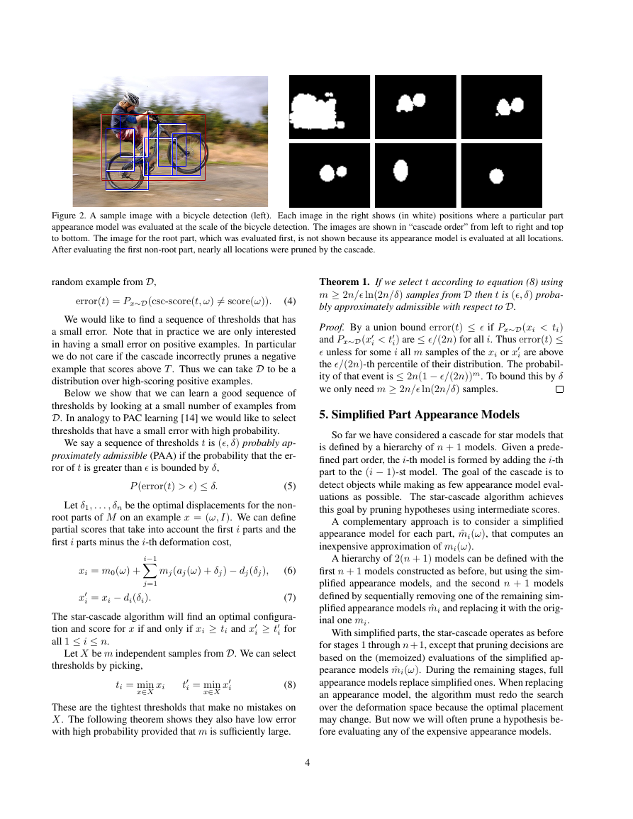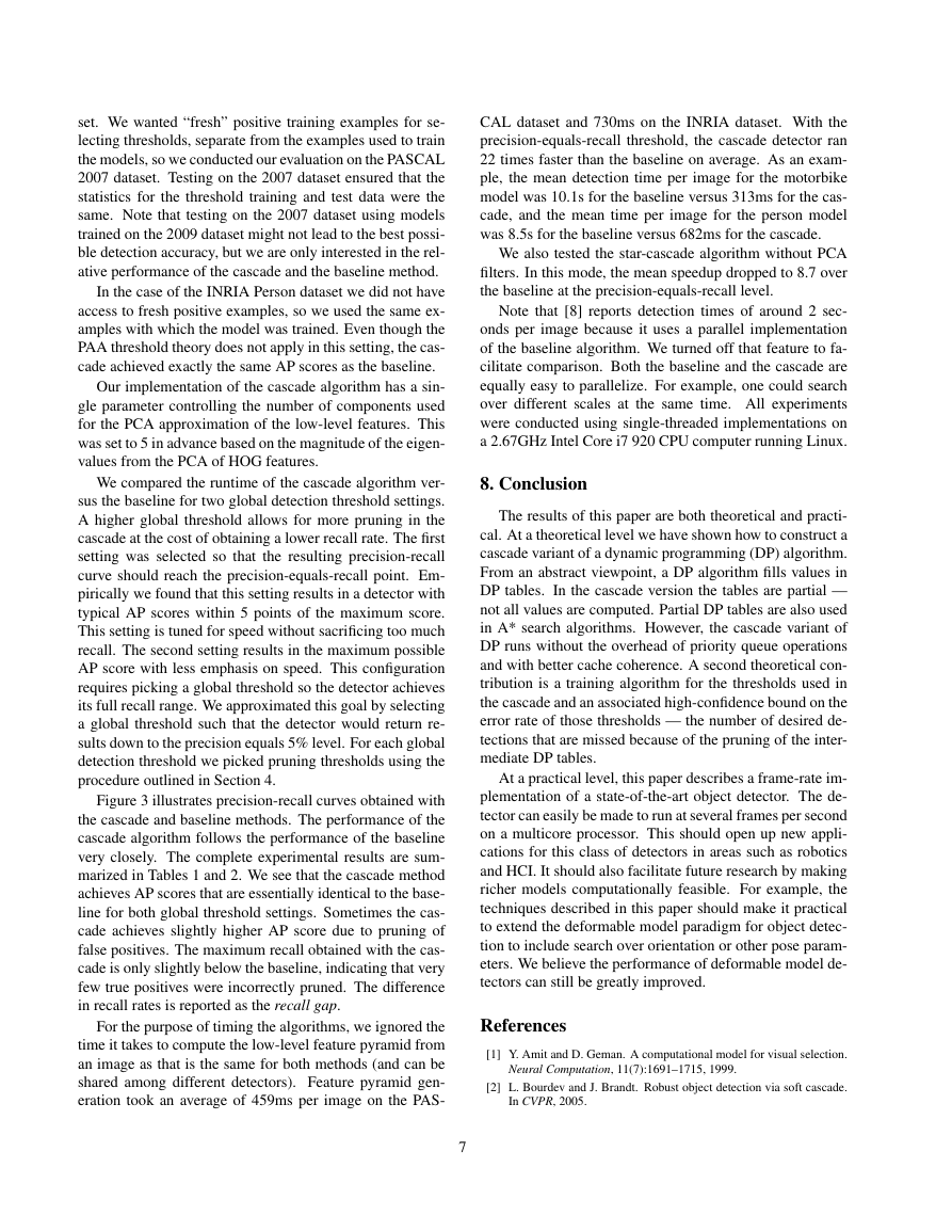Figure 3 illustrates precision-recall curves obtained with the cascade and baseline methods. 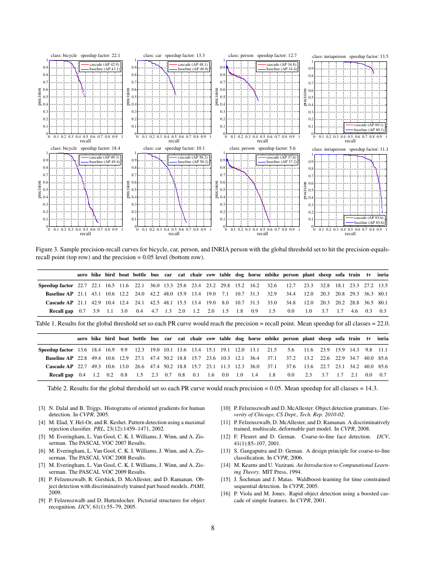The performance of the cascade algorithm follows the performance of the baseline very closely. The complete experimental results are sum- marized in Tables 1 and 2. We see that the cascade method achieves AP scores that are essentially identical to the base- line for both global threshold settings. Sometimes the cas- cade achieves slightly higher AP score due to pruning of false positives. The maximum recall obtained with the cas- cade is only slightly below the baseline, indicating that very few true positives were incorrectly pruned. The difference in recall rates is reported as the recall gap. For the purpose of timing the algorithms, we ignored the time it takes to compute the low-level feature pyramid from an image as that is the same for both methods (and can be shared among different detectors). Feature pyramid gen- eration took an average of 459ms per image on the PAS- CAL dataset and 730ms on the INRIA dataset. With the precision-equals-recall threshold, the cascade detector ran 22 times faster than the baseline on average. As an exam- ple, the mean detection time per image for the motorbike model was 10.1s for the baseline versus 313ms for the cas- cade, and the mean time per image for the person model was 8.5s for the baseline versus 682ms for the cascade. We also tested the star-cascade algorithm without PCA ﬁlters. In this mode, the mean speedup dropped to 8.7 over the baseline at the precision-equals-recall level. Note that [8] reports detection times of around 2 sec- onds per image because it uses a parallel implementation of the baseline algorithm. We turned off that feature to fa- cilitate comparison. Both the baseline and the cascade are equally easy to parallelize. For example, one could search over different scales at the same time. All experiments were conducted using single-threaded implementations on a 2.67GHz Intel Core i7 920 CPU computer running Linux. 8. Conclusion The results of this paper are both theoretical and practi- cal. At a theoretical level we have shown how to construct a cascade variant of a dynamic programming (DP) algorithm. From an abstract viewpoint, a DP algorithm ﬁlls values in DP tables. In the cascade version the tables are partial — not all values are computed. Partial DP tables are also used in A* search algorithms. However, the cascade variant of DP runs without the overhead of priority queue operations and with better cache coherence. A second theoretical con- tribution is a training algorithm for the thresholds used in the cascade and an associated high-conﬁdence bound on the error rate of those thresholds — the number of desired de- tections that are missed because of the pruning of the inter- mediate DP tables. At a practical level, this paper describes a frame-rate im- plementation of a state-of-the-art object detector. The de- tector can easily be made to run at several frames per second on a multicore processor. This should open up new appli- cations for this class of detectors in areas such as robotics and HCI. It should also facilitate future research by making richer models computationally feasible. For example, the techniques described in this paper should make it practical to extend the deformable model paradigm for object detec- tion to include search over orientation or other pose param- eters. We believe the performance of deformable model de- tectors can still be greatly improved. References [1] Y. Amit and D. Geman. A computational model for visual selection. Neural Computation, 11(7):1691–1715, 1999. [2] L. Bourdev and J. Brandt. Robust object detection via soft cascade. In CVPR, 2005. 7

Figure 3. Sample precision-recall curves for bicycle, car, person, and INRIA person with the global threshold set to hit the precision-equals- recall point (top row) and the precision = 0.05 level (bottom row). aero bike bird boat bottle bus car cat chair cow table dog horse mbike person plant sheep sofa train tv inria Speedup factor 22.7 22.1 16.5 11.6 Baseline AP 21.1 43.1 10.6 12.2 Cascade AP 21.1 42.9 10.4 12.4 3.0 Recall gap 0.7 3.9 1.1 22.1 24.0 24.1 0.4 36.0 13.3 25.6 23.4 23.2 29.8 15.2 10.7 42.2 48.0 15.9 13.4 19.0 10.7 42.5 48.1 15.5 13.4 19.0 4.7 2.0 1.8 7.1 8.0 1.5 2.0 1.3 1.2 16.2 31.3 31.3 0.9 32.6 32.9 33.0 1.5 12.7 34.4 34.8 0.0 23.3 12.0 12.0 1.0 32.8 20.3 20.3 3.7 18.1 23.3 27.2 13.5 20.8 29.3 36.3 80.1 20.2 28.8 36.5 80.1 1.7 0.3 4.6 0.3 Table 1. Results for the global threshold set so each PR curve would reach the precision = recall point. Mean speedup for all classes = 22.0. aero bike bird boat bottle bus car cat chair cow table dog horse mbike person plant sheep sofa train tv inria Speedup factor 13.6 18.4 16.9 9.9 Baseline AP 22.8 49.4 10.6 12.9 Cascade AP 22.7 49.3 10.6 13.0 0.8 Recall gap 0.4 1.2 0.2 12.3 27.1 26.6 1.5 19.0 10.1 13.6 13.4 15.1 19.1 12.0 47.4 50.2 18.8 15.7 23.6 10.3 12.1 47.4 50.2 18.8 15.7 23.1 11.3 12.3 2.3 1.0 0.8 0.0 0.7 0.1 1.6 13.1 36.4 36.0 1.4 21.5 37.1 37.1 1.8 5.6 37.2 37.6 0.0 11.6 13.2 13.6 2.3 23.9 22.6 22.7 3.7 9.8 15.9 14.3 11.1 22.9 34.7 40.0 85.6 23.1 34.2 40.0 85.6 1.7 0.7 2.1 0.0 Table 2. Results for the global threshold set so each PR curve would reach precision = 0.05. Mean speedup for all classes = 14.3. [3] N. Dalal and B. Triggs. Histograms of oriented gradients for human detection. In CVPR, 2005. [4] M. Elad, Y. Hel-Or, and R. Keshet. Pattern detection using a maximal rejection classiﬁer. PRL, 23(12):1459–1471, 2002. [5] M. Everingham, L. Van Gool, C. K. I. Williams, J. Winn, and A. Zis- serman. The PASCAL VOC 2007 Results. [6] M. Everingham, L. Van Gool, C. K. I. Williams, J. Winn, and A. Zis- serman. The PASCAL VOC 2008 Results. [7] M. Everingham, L. Van Gool, C. K. I. Williams, J. Winn, and A. Zis- serman. The PASCAL VOC 2009 Results. [8] P. Felzenszwalb, R. Girshick, D. McAllester, and D. Ramanan. Ob- ject detection with discriminatively trained part based models. PAMI, 2009. [9] P. Felzenszwalb and D. Huttenlocher. Pictorial structures for object recognition. IJCV, 61(1):55–79, 2005. 8 [10] P. Felzenszwalb and D. McAllester. Object detection grammars. Uni- verity of Chicago, CS Dept., Tech. Rep. 2010-02. [11] P. Felzenszwalb, D. McAllester, and D. Ramanan. A discriminatively trained, multiscale, deformable part model. In CVPR, 2008. [12] F. Fleuret and D. Geman. Coarse-to-ﬁne face detection. IJCV, 41(1):85–107, 2001. [13] S. Gangaputra and D. Geman. A design principle for coarse-to-ﬁne classiﬁcation. In CVPR, 2006. [14] M. Kearns and U. Vazirani. An Introduction to Computational Learn- ing Theory. MIT Press, 1994. [15] J. ˇSochman and J. Matas. Waldboost-learning for time constrained sequential detection. In CVPR, 2005. [16] P. Viola and M. Jones. Rapid object detection using a boosted cas- cade of simple features. In CVPR, 2001. 00.10.20.30.40.50.60.70.80.9100.10.20.30.40.50.60.70.80.91recallprecisionclass: bicycle speedup factor: 22.1 cascade (AP 42.9)baseline (AP 43.1)00.10.20.30.40.50.60.70.80.9100.10.20.30.40.50.60.70.80.91recallprecisionclass: car speedup factor: 13.3 cascade (AP 48.1)baseline (AP 48.0)00.10.20.30.40.50.60.70.80.9100.10.20.30.40.50.60.70.80.91recallprecisionclass: person speedup factor: 12.7 cascade (AP 34.8)baseline (AP 34.4)00.10.20.30.40.50.60.70.80.9100.10.20.30.40.50.60.70.80.91recallprecisionclass: inriaperson speedup factor: 13.5 cascade (AP 80.1)baseline (AP 80.1)00.10.20.30.40.50.60.70.80.9100.10.20.30.40.50.60.70.80.91recallprecisionclass: bicycle speedup factor: 18.4 cascade (AP 49.3)baseline (AP 49.4)00.10.20.30.40.50.60.70.80.9100.10.20.30.40.50.60.70.80.91recallprecisionclass: car speedup factor: 10.1 cascade (AP 50.2)baseline (AP 50.2)00.10.20.30.40.50.60.70.80.9100.10.20.30.40.50.60.70.80.91recallprecisionclass: person speedup factor: 5.6 cascade (AP 37.6)baseline (AP 37.2)00.10.20.30.40.50.60.70.80.9100.10.20.30.40.50.60.70.80.91recallprecisionclass: inriaperson speedup factor: 11.1 cascade (AP 85.6)baseline (AP 85.6)

分享到：

赞收藏

资料库

Cascade Object Detection with Deformable Part Models_CVPR2010.pdf

相关推荐

开发技术

热门标签

最新资料