Sequential Minimal Optimization:
A Fast Algorithm for Training Support Vector Machines
John C. Platt
Microsoft Research
jplatt@microsoft.com
Technical Report MSR-TR-98-14
April 21, 1998
© 1998 John Platt
ABSTRACT
This paper proposes a new algorithm for training support vector machines: Sequential
Minimal Optimization, or SMO. Training a support vector machine requires the solution of
a very large quadratic programming (QP) optimization problem. SMO breaks this large
QP problem into a series of smallest possible QP problems. These small QP problems are
solved analytically, which avoids using a time-consuming numerical QP optimization as an
inner loop. The amount of memory required for SMO is linear in the training set size,
which allows SMO to handle very large training sets. Because matrix computation is
avoided, SMO scales somewhere between linear and quadratic in the training set size for
various test problems, while the standard chunking SVM algorithm scales somewhere
between linear and cubic in the training set size. SMO’s computation time is dominated by
SVM evaluation, hence SMO is fastest for linear SVMs and sparse data sets. On real-
world sparse data sets, SMO can be more than 1000 times faster than the chunking
algorithm.
1. INTRODUCTION
In the last few years, there has been a surge of interest in Support Vector Machines (SVMs) [19]
[20] [4]. SVMs have empirically been shown to give good generalization performance on a wide
variety of problems such as handwritten character recognition [12], face detection [15], pedestrian
detection [14], and text categorization [9].
However, the use of SVMs is still limited to a small group of researchers. One possible reason is
that training algorithms for SVMs are slow, especially for large problems. Another explanation is
that SVM training algorithms are complex, subtle, and difficult for an average engineer to
implement.
This paper describes a new SVM learning algorithm that is conceptually simple, easy to
implement, is generally faster, and has better scaling properties for difficult SVM problems than
the standard SVM training algorithm. The new SVM learning algorithm is called Sequential
Minimal Optimization (or SMO). Instead of previous SVM learning algorithms that use
numerical quadratic programming (QP) as an inner loop, SMO uses an analytic QP step.
This paper first provides an overview of SVMs and a review of current SVM training algorithms.
The SMO algorithm is then presented in detail, including the solution to the analytic QP step,
1
�
heuristics for choosing which variables to optimize in the inner loop, a description of how to set
the threshold of the SVM, some optimizations for special cases, the pseudo-code of the algorithm,
and the relationship of SMO to other algorithms.
SMO has been tested on two real-world data sets and two artificial data sets. This paper presents
the results for timing SMO versus the standard “chunking” algorithm for these data sets and
presents conclusions based on these timings. Finally, there is an appendix that describes the
derivation of the analytic optimization.
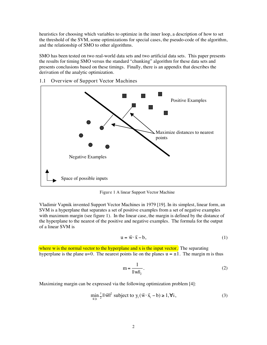
1.1 Overview of Support Vector Machines
Positive Examples
Maximize distances to nearest
points
Negative Examples
Space of possible inputs
Figure 1 A linear Support Vector Machine
Vladimir Vapnik invented Support Vector Machines in 1979 [19]. In its simplest, linear form, an
SVM is a hyperplane that separates a set of positive examples from a set of negative examples
with maximum margin (see figure 1). In the linear case, the margin is defined by the distance of
the hyperplane to the nearest of the positive and negative examples. The formula for the output
of a linear SVM is
r r
=
u w x b
,
(1)
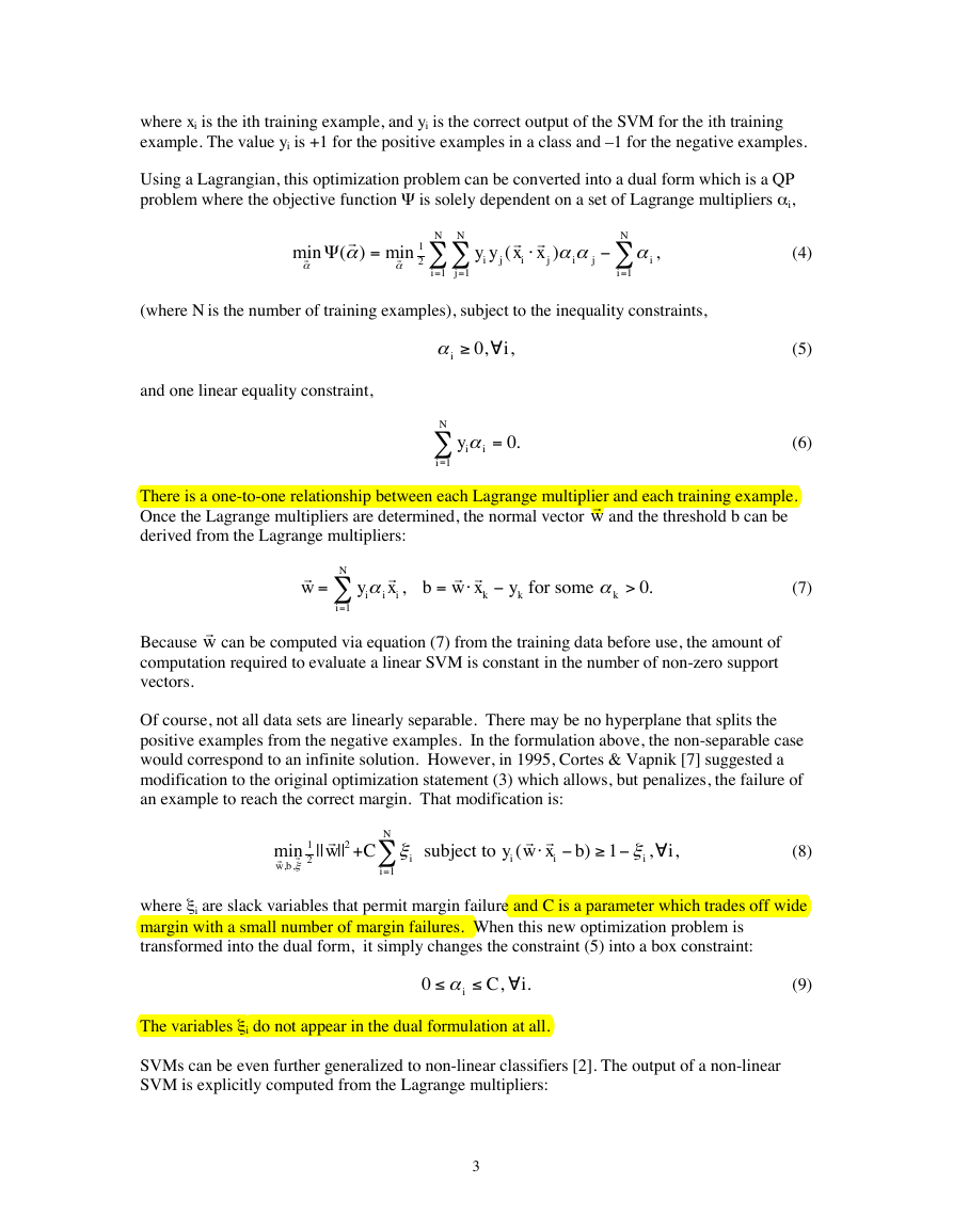
where w is the normal vector to the hyperplane and x is the input vector. The separating
hyperplane is the plane u=0. The nearest points lie on the planes u = – 1. The margin m is thus
m
= 1
||
w
2
||
.
Maximizing margin can be expressed via the following optimization problem [4]:
r
2
||
w
min ||
,r
w b
1
2
subject to
r r
y w x
i
i
(
b
)
,
1
i
,
(2)
(3)
2
-
-
‡
"
�
where xi is the ith training example, and yi is the correct output of the SVM for the ith training
example. The value yi is +1 for the positive examples in a class and –1 for the negative examples.
Using a Lagrangian, this optimization problem can be converted into a dual form which is a QP
problem where the objective function Y
i,
is solely dependent on a set of Lagrange multipliers a
r
a
=
) min
min (
a
a
r
r
1
2
N
N
=
1
i
=
1
j
r
y y x x
i
r
i
(
j
aa
)
j
i
j
a
N
=
1
i
,
i
(where N is the number of training examples), subject to the inequality constraints,
and one linear equality constraint,
a
i
"0,
i
,
a
yi
i
=
0
.
N
=
1
i
(4)
(5)
(6)
There is a one-to-one relationship between each Lagrange multiplier and each training example.
r
w and the threshold b can be
Once the Lagrange multipliers are determined, the normal vector
derived from the Lagrange multipliers:
r
w
=
N
=
1
i
a
y
i
r
x
i
i
,
r r
b w x
k
=
a
for some
y
k
>
k
0
.
(7)
r
w can be computed via equation (7) from the training data before use, the amount of
Because
computation required to evaluate a linear SVM is constant in the number of non-zero support
vectors.
Of course, not all data sets are linearly separable. There may be no hyperplane that splits the
positive examples from the negative examples. In the formulation above, the non-separable case
would correspond to an infinite solution. However, in 1995, Cortes & Vapnik [7] suggested a
modification to the original optimization statement (3) which allows, but penalizes, the failure of
an example to reach the correct margin. That modification is:
min ||
,
w b
x
,
1
2
r
r
r
2
||
w
+
C
x
i
N
=
1
i
subject to
r r
y w x
i
i
(
b
)
x
1
,
i
i
,
(8)
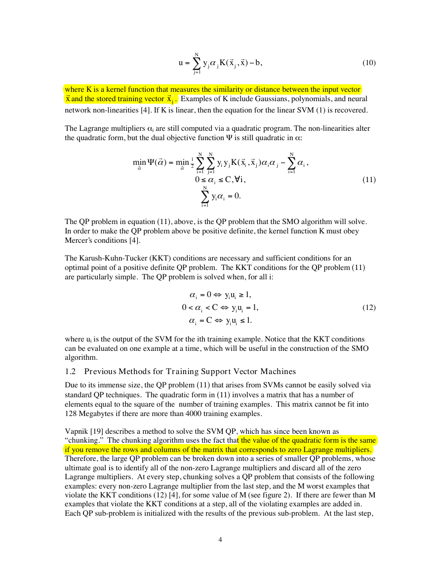
i are slack variables that permit margin failure and C is a parameter which trades off wide
where x
margin with a small number of margin failures. When this new optimization problem is
transformed into the dual form, it simply changes the constraint (5) into a box constraint:
0 £
a
i C i
,
.
(9)
The variables x
i do not appear in the dual formulation at all.
SVMs can be even further generalized to non-linear classifiers [2]. The output of a non-linear
SVM is explicitly computed from the Lagrange multipliers:
3
Y
-
‡
-
-
‡
-
"
£
"
�
=
u
a
y
j
j
N
=
1
j
r
r
K x x
(
,
j
)
b
,
(10)
where K is a kernel function that measures the similarity or distance between the input vector
r
r
x and the stored training vector
x j . Examples of K include Gaussians, polynomials, and neural
network non-linearities [4]. If K is linear, then the equation for the linear SVM (1) is recovered.
The Lagrange multipliers a
the quadratic form, but the dual objective function Y
i are still computed via a quadratic program. The non-linearities alter
is still quadratic in a:
r
a
=
) min
min (
a
a
r
r
1
2
N
N
r r
y y K x x
i
i
(
,
j
=
1
i
0
j
=
1
a
i
a
y
i
i
N
=
1
i
,
,
C i
=
.
0
aa
)
j
i
j
a
N
=
1
i
,
i
(11)
The QP problem in equation (11), above, is the QP problem that the SMO algorithm will solve.
In order to make the QP problem above be positive definite, the kernel function K must obey
Mercer’s conditions [4].
The Karush-Kuhn-Tucker (KKT) conditions are necessary and sufficient conditions for an
optimal point of a positive definite QP problem. The KKT conditions for the QP problem (11)
are particularly simple. The QP problem is solved when, for all i:
a
<
a
i
a
i
0
=
0
<
C
C
=
i
y u
i
i
=
y u
i
i
y u
i
i
1
,
1
.
1
,
(12)
where ui is the output of the SVM for the ith training example. Notice that the KKT conditions
can be evaluated on one example at a time, which will be useful in the construction of the SMO
algorithm.
1.2 Previous Methods for Training Support Vector Machines
Due to its immense size, the QP problem (11) that arises from SVMs cannot be easily solved via
standard QP techniques. The quadratic form in (11) involves a matrix that has a number of
elements equal to the square of the number of training examples. This matrix cannot be fit into
128 Megabytes if there are more than 4000 training examples.
Vapnik [19] describes a method to solve the SVM QP, which has since been known as
“chunking.” The chunking algorithm uses the fact that the value of the quadratic form is the same
if you remove the rows and columns of the matrix that corresponds to zero Lagrange multipliers.
Therefore, the large QP problem can be broken down into a series of smaller QP problems, whose
ultimate goal is to identify all of the non-zero Lagrange multipliers and discard all of the zero
Lagrange multipliers. At every step, chunking solves a QP problem that consists of the following
examples: every non-zero Lagrange multiplier from the last step, and the M worst examples that
violate the KKT conditions (12) [4], for some value of M (see figure 2). If there are fewer than M
examples that violate the KKT conditions at a step, all of the violating examples are added in.
Each QP sub-problem is initialized with the results of the previous sub-problem. At the last step,
4
-
Y
-
£
£
"
‡
£
�
the entire set of non-zero Lagrange multipliers has been identified, hence the last step solves the
large QP problem.
Chunking seriously reduces the size of the matrix from the number of training examples squared
to approximately the number of non-zero Lagrange multipliers squared. However, chunking still
cannot handle large-scale training problems, since even this reduced matrix cannot fit into
memory.
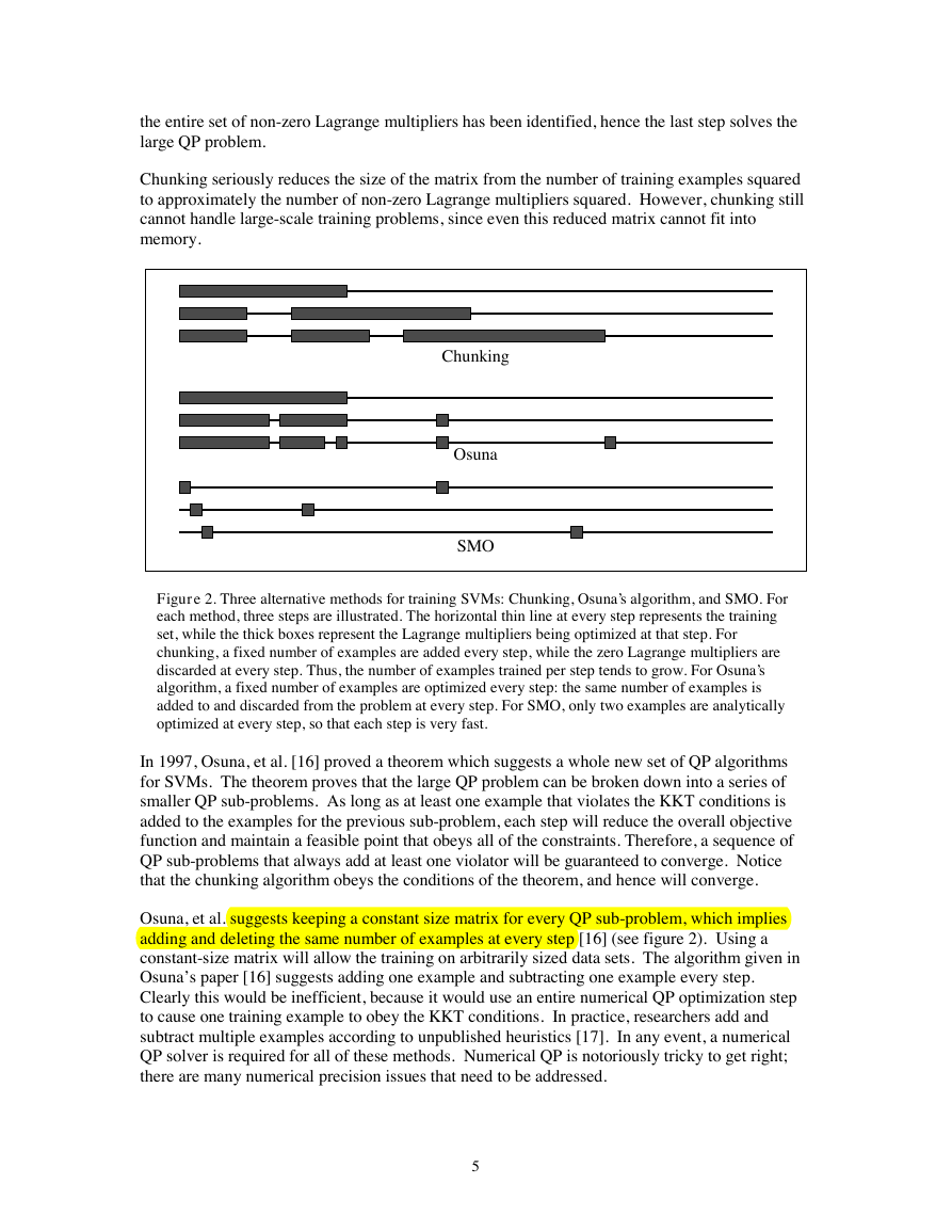
Chunking
Osuna
SMO
Figure 2. Three alternative methods for training SVMs: Chunking, Osuna’s algorithm, and SMO. For
each method, three steps are illustrated. The horizontal thin line at every step represents the training
set, while the thick boxes represent the Lagrange multipliers being optimized at that step. For
chunking, a fixed number of examples are added every step, while the zero Lagrange multipliers are
discarded at every step. Thus, the number of examples trained per step tends to grow. For Osuna’s
algorithm, a fixed number of examples are optimized every step: the same number of examples is
added to and discarded from the problem at every step. For SMO, only two examples are analytically
optimized at every step, so that each step is very fast.
In 1997, Osuna, et al. [16] proved a theorem which suggests a whole new set of QP algorithms
for SVMs. The theorem proves that the large QP problem can be broken down into a series of
smaller QP sub-problems. As long as at least one example that violates the KKT conditions is
added to the examples for the previous sub-problem, each step will reduce the overall objective
function and maintain a feasible point that obeys all of the constraints. Therefore, a sequence of
QP sub-problems that always add at least one violator will be guaranteed to converge. Notice
that the chunking algorithm obeys the conditions of the theorem, and hence will converge.
Osuna, et al. suggests keeping a constant size matrix for every QP sub-problem, which implies
adding and deleting the same number of examples at every step [16] (see figure 2). Using a
constant-size matrix will allow the training on arbitrarily sized data sets. The algorithm given in
Osuna’s paper [16] suggests adding one example and subtracting one example every step.
Clearly this would be inefficient, because it would use an entire numerical QP optimization step
to cause one training example to obey the KKT conditions. In practice, researchers add and
subtract multiple examples according to unpublished heuristics [17]. In any event, a numerical
QP solver is required for all of these methods. Numerical QP is notoriously tricky to get right;
there are many numerical precision issues that need to be addressed.
5
�
2. SEQUENTIAL MINIMAL OPTIMIZATION
Sequential Minimal Optimization (SMO) is a simple algorithm that can quickly solve the SVM
QP problem without any extra matrix storage and without using numerical QP optimization steps
at all. SMO decomposes the overall QP problem into QP sub-problems, using Osuna’s theorem
to ensure convergence.
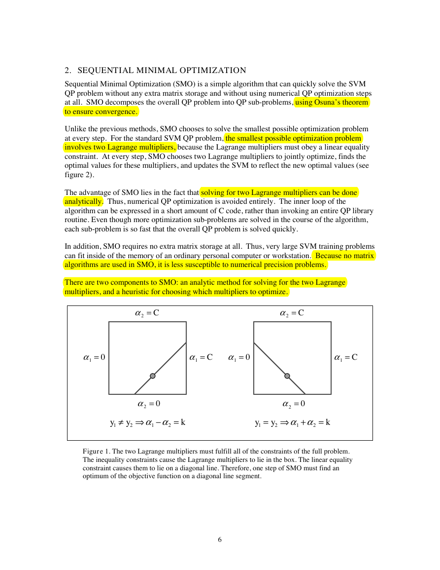
Unlike the previous methods, SMO chooses to solve the smallest possible optimization problem
at every step. For the standard SVM QP problem, the smallest possible optimization problem
involves two Lagrange multipliers, because the Lagrange multipliers must obey a linear equality
constraint. At every step, SMO chooses two Lagrange multipliers to jointly optimize, finds the
optimal values for these multipliers, and updates the SVM to reflect the new optimal values (see
figure 2).
The advantage of SMO lies in the fact that solving for two Lagrange multipliers can be done
analytically. Thus, numerical QP optimization is avoided entirely. The inner loop of the
algorithm can be expressed in a short amount of C code, rather than invoking an entire QP library
routine. Even though more optimization sub-problems are solved in the course of the algorithm,
each sub-problem is so fast that the overall QP problem is solved quickly.
In addition, SMO requires no extra matrix storage at all. Thus, very large SVM training problems
can fit inside of the memory of an ordinary personal computer or workstation. Because no matrix
algorithms are used in SMO, it is less susceptible to numerical precision problems.
There are two components to SMO: an analytic method for solving for the two Lagrange
multipliers, and a heuristic for choosing which multipliers to optimize.
a
2
= C
a
2
= C
a
1
0=
a
1
= C
a
1
0=
a
1
= C
a
0=
¡ ˘ -
a a
2
y
2
1
y
1
=
k
2
y
1
a
0=
= ˘ +
a a
2
y
2
1
=
k
2
Figure 1. The two Lagrange multipliers must fulfill all of the constraints of the full problem.
The inequality constraints cause the Lagrange multipliers to lie in the box. The linear equality
constraint causes them to lie on a diagonal line. Therefore, one step of SMO must find an
optimum of the objective function on a diagonal line segment.
6
�
2.1 Solving for Two Lagrange Multipliers
In order to solve for the two Lagrange multipliers, SMO first computes the constraints on these
multipliers and then solves for the constrained minimum. For convenience, all quantities that
refer to the first multiplier will have a subscript 1, while all quantities that refer to the second
multiplier will have a subscript 2. Because there are only two multipliers, the constraints can be
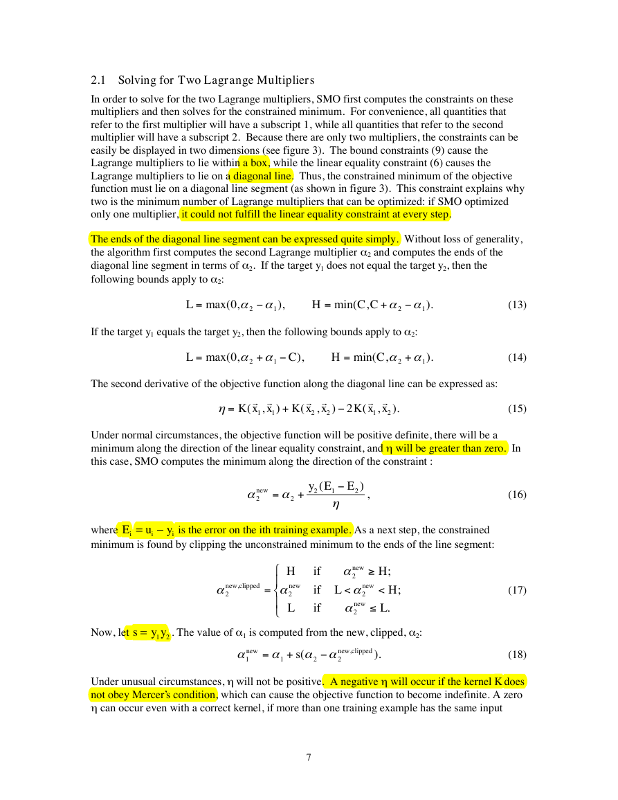
easily be displayed in two dimensions (see figure 3). The bound constraints (9) cause the
Lagrange multipliers to lie within a box, while the linear equality constraint (6) causes the
Lagrange multipliers to lie on a diagonal line. Thus, the constrained minimum of the objective
function must lie on a diagonal line segment (as shown in figure 3). This constraint explains why
two is the minimum number of Lagrange multipliers that can be optimized: if SMO optimized
only one multiplier, it could not fulfill the linear equality constraint at every step.
The ends of the diagonal line segment can be expressed quite simply. Without loss of generality,
the algorithm first computes the second Lagrange multiplier a
diagonal line segment in terms of a
following bounds apply to a 2:
2. If the target y1 does not equal the target y2, then the
2 and computes the ends of the
=
L
max( ,
0
a
2
a
),
1
=
H
min(
+
C C
,
a
2
If the target y1 equals the target y2, then the following bounds apply to a
+
=
+
a
a
a
L
max( ,
0
=
H
2
1
C
),
min(
C
,
2
a
2:
a
).
1
).
1
The second derivative of the objective function along the diagonal line can be expressed as:
h =
r r
K x x
1
1
(
,
+
)
r
K x x
2
r
2
(
,
)
2
r r
K x x
2
1
(
,
).
(13)
(14)
(15)
Under normal circumstances, the objective function will be positive definite, there will be a
minimum along the direction of the linear equality constraint, and h will be greater than zero. In
this case, SMO computes the minimum along the direction of the constraint :
a
a
new =
2
+
2
y E
2
1
(
h
E
2
)
,
=
- is the error on the ith training example. As a next step, the constrained
where E
minimum is found by clipping the unconstrained minimum to the ends of the line segment:
u
i
y
i
i
a
new,clipped
2
=
%
&K
a
’K
H
new
2
L
if
if
if
a
<
a
a
new
2
new
2
new
2
L
;
H
<
H
.
L
;
(16)
(17)
(18)
Now, let s
=
1 2 . The value of a
y y
1 is computed from the new, clipped, a 2:
a
new
1
=
a
+
a
s(
1
2
a
new,clipped
2
).
will not be positive. A negative h will occur if the kernel K does
Under unusual circumstances, h
not obey Mercer’s condition, which can cause the objective function to become indefinite. A zero
h can occur even with a correct kernel, if more than one training example has the same input
7
-
-
-
-
-
‡
£
-
�
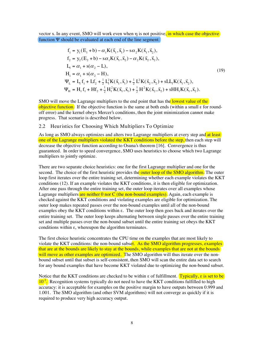
vector x. In any event, SMO will work even when h
function Y
should be evaluated at each end of the line segment:
is not positive, in which case the objective
=
=
=
=
=
=
1
f
f
2
L
1
H
1
L
H
1
+
)
(
y E b
1
1
+
(
)
b
y E
2
2
+
a
a
(
s
+
a
a
(
s
2
1
+
L f
Lf
2
1 1
+
H f Hf
2
1 1
2
1
)
(
r r
a
,
)
K x x
1
1
1
r r
a
,
(
s K x x
1
2
),
L
),
H
r r
1
2
,
)
L K x x
1
1
1
2
r r
1
,
(
H K x x
1
1
2
2
1
(
+
+
r r
a
(
s K x x
1
2
r
r
a
,
(
K x x
2
2
,
2
2
),
),
1
2
+
r
2
,
L K x x
2
r
1
,
2
2
r r
+
,
)
),
sLL K x x
2
1
1
r
r r
+
(
)
,
H K x x
sHH K x x
2
1
2
r
2
(
(
2
(
1
(19)
).
+
)
SMO will move the Lagrange multipliers to the end point that has the lowest value of the
objective function. If the objective function is the same at both ends (within a small e for round-
off error) and the kernel obeys Mercer’s conditions, then the joint minimization cannot make
progress. That scenario is described below.
2.2 Heuristics for Choosing Which Multipliers To Optimize
As long as SMO always optimizes and alters two Lagrange multipliers at every step and at least
one of the Lagrange multipliers violated the KKT conditions before the step, then each step will
decrease the objective function according to Osuna’s theorem [16]. Convergence is thus
guaranteed. In order to speed convergence, SMO uses heuristics to choose which two Lagrange
multipliers to jointly optimize.
There are two separate choice heuristics: one for the first Lagrange multiplier and one for the
second. The choice of the first heuristic provides the outer loop of the SMO algorithm. The outer
loop first iterates over the entire training set, determining whether each example violates the KKT
conditions (12). If an example violates the KKT conditions, it is then eligible for optimization.
After one pass through the entire training set, the outer loop iterates over all examples whose
Lagrange multipliers are neither 0 nor C (the non-bound examples). Again, each example is
checked against the KKT conditions and violating examples are eligible for optimization. The
outer loop makes repeated passes over the non-bound examples until all of the non-bound
examples obey the KKT conditions within e. The outer loop then goes back and iterates over the
entire training set. The outer loop keeps alternating between single passes over the entire training
set and multiple passes over the non-bound subset until the entire training set obeys the KKT
conditions within e, whereupon the algorithm terminates.
The first choice heuristic concentrates the CPU time on the examples that are most likely to
violate the KKT conditions: the non-bound subset. As the SMO algorithm progresses, examples
that are at the bounds are likely to stay at the bounds, while examples that are not at the bounds
will move as other examples are optimized. The SMO algorithm will thus iterate over the non-
bound subset until that subset is self-consistent, then SMO will scan the entire data set to search
for any bound examples that have become KKT violated due to optimizing the non-bound subset.
Notice that the KKT conditions are checked to be within e of fulfillment. Typically, e is set to be
10-3. Recognition systems typically do not need to have the KKT conditions fulfilled to high
accuracy: it is acceptable for examples on the positive margin to have outputs between 0.999 and
1.001. The SMO algorithm (and other SVM algorithms) will not converge as quickly if it is
required to produce very high accuracy output.
8
-
-
-
-
-
-
Y
Y
�



 2023年江西萍乡中考道德与法治真题及答案.doc
 2012年重庆南川中考生物真题及答案.doc
 2013年江西师范大学地理学综合及文艺理论基础考研真题.doc
 2020年四川甘孜小升初语文真题及答案I卷.doc
 2020年注册岩土工程师专业基础考试真题及答案.doc
 2023-2024学年福建省厦门市九年级上学期数学月考试题及答案.doc
 2021-2022学年辽宁省沈阳市大东区九年级上学期语文期末试题及答案.doc
 2022-2023学年北京东城区初三第一学期物理期末试卷及答案.doc
 2018上半年江西教师资格初中地理学科知识与教学能力真题及答案.doc
 2012年河北国家公务员申论考试真题及答案-省级.doc
 2020-2021学年江苏省扬州市江都区邵樊片九年级上学期数学第一次质量检测试题及答案.doc
 2022下半年黑龙江教师资格证中学综合素质真题及答案.doc