Knowl Inf Syst (2008) 14:1–37
DOI 10.1007/s10115-007-0114-2
SURVEY PAPER
Top 10 algorithms in data mining
Xindong Wu · Vipin Kumar · J. Ross Quinlan · Joydeep Ghosh · Qiang Yang ·
Hiroshi Motoda · Geoffrey J. McLachlan · Angus Ng · Bing Liu · Philip S. Yu ·
Zhi-Hua Zhou · Michael Steinbach · David J. Hand · Dan Steinberg
Received: 9 July 2007 / Revised: 28 September 2007 / Accepted: 8 October 2007
Published online: 4 December 2007
© Springer-Verlag London Limited 2007
Abstract This paper presents the top 10 data mining algorithms identified by the IEEE
International Conference on Data Mining (ICDM) in December 2006: C4.5, k-Means, SVM,
Apriori, EM, PageRank, AdaBoost, kNN, Naive Bayes, and CART. These top 10 algorithms
are among the most influential data mining algorithms in the research community. With each
algorithm, we provide a description of the algorithm, discuss the impact of the algorithm, and
review current and further research on the algorithm. These 10 algorithms cover classification,
X. Wu (B)
Department of Computer Science, University of Vermont, Burlington, VT, USA
e-mail: xwu@cs.uvm.edu
V. Kumar
Department of Computer Science and Engineering,
University of Minnesota, Minneapolis, MN, USA
e-mail: kumar@cs.umn.edu
J. Ross Quinlan
Rulequest Research Pty Ltd,
St Ives, NSW, Australia
e-mail: quinlan@rulequest.com
J. Ghosh
Department of Electrical and Computer Engineering,
University of Texas at Austin, Austin, TX 78712, USA
e-mail: ghosh@ece.utexas.edu
Q. Yang
Department of Computer Science,
Hong Kong University of Science and Technology,
Honkong, China
e-mail: qyang@cs.ust.hk
H. Motoda
AFOSR/AOARD and Osaka University,
7-23-17 Roppongi, Minato-ku, Tokyo 106-0032, Japan
e-mail: motoda@ar.sanken.osaka-u.ac.jp
123
�
2
X. Wu et al.
clustering, statistical learning, association analysis, and link mining, which are all among the
most important topics in data mining research and development.
0 Introduction
In an effort to identify some of the most influential algorithms that have been widely used
in the data mining community, the IEEE International Conference on Data Mining (ICDM,
http://www.cs.uvm.edu/~icdm/) identified the top 10 algorithms in data mining for presen-
tation at ICDM ’06 in Hong Kong.
As the first step in the identification process, in September 2006 we invited the ACM KDD
Innovation Award and IEEE ICDM Research Contributions Award winners to each nomi-
nate up to 10 best-known algorithms in data mining. All except one in this distinguished
set of award winners responded to our invitation. We asked each nomination to provide the
following information: (a) the algorithm name, (b) a brief justification, and (c) a representa-
tive publication reference. We also advised that each nominated algorithm should have been
widely cited and used by other researchers in the field, and the nominations from each nomi-
nator as a group should have a reasonable representation of the different areas in data mining.
G. J. McLachlan
Department of Mathematics,
The University of Queensland, Brisbane, Australia
e-mail: gjm@maths.uq.edu.au
A. Ng
School of Medicine, Griffith University,
Brisbane, Australia
B. Liu
Department of Computer Science,
University of Illinois at Chicago, Chicago, IL 60607, USA
P. S. Yu
IBM T. J. Watson Research Center,
Hawthorne, NY 10532, USA
e-mail: psyu@us.ibm.com
Z.-H. Zhou
National Key Laboratory for Novel Software Technology,
Nanjing University, Nanjing 210093, China
e-mail: zhouzh@nju.edu.cn
M. Steinbach
Department of Computer Science and Engineering,
University of Minnesota, Minneapolis, MN 55455, USA
e-mail: steinbac@cs.umn.edu
D. J. Hand
Department of Mathematics,
Imperial College, London, UK
e-mail: d.j.hand@imperial.ac.uk
D. Steinberg
Salford Systems,
San Diego, CA 92123, USA
e-mail: dsx@salford-systems.com
123
�
Top 10 algorithms in data mining
3
After the nominations in Step 1, we verified each nomination for its citations on Google
Scholar in late October 2006, and removed those nominations that did not have at least 50
citations. All remaining (18) nominations were then organized in 10 topics: association anal-
ysis, classification, clustering, statistical learning, bagging and boosting, sequential patterns,
integrated mining, rough sets, link mining, and graph mining. For some of these 18 algorithms
such as k-means, the representative publication was not necessarily the original paper that
introduced the algorithm, but a recent paper that highlights the importance of the technique.
These representative publications are available at the ICDM website (http://www.cs.uvm.
edu/~icdm/algorithms/CandidateList.shtml).
In the third step of the identification process, we had a wider involvement of the research
community. We invited the Program Committee members of KDD-06 (the 2006 ACM SIG-
KDD International Conference on Knowledge Discovery and Data Mining), ICDM ’06 (the
2006 IEEE International Conference on Data Mining), and SDM ’06 (the 2006 SIAM Inter-
national Conference on Data Mining), as well as the ACM KDD Innovation Award and IEEE
ICDM Research Contributions Award winners to each vote for up to 10 well-known algo-
rithms from the 18-algorithm candidate list. The voting results of this step were presented at
the ICDM ’06 panel on Top 10 Algorithms in Data Mining.
At the ICDM ’06 panel of December 21, 2006, we also took an open vote with all 145
attendees on the top 10 algorithms from the above 18-algorithm candidate list, and the top 10
algorithms from this open vote were the same as the voting results from the above third step.
The 3-hour panel was organized as the last session of the ICDM ’06 conference, in parallel
with 7 paper presentation sessions of the Web Intelligence (WI ’06) and Intelligent Agent
Technology (IAT ’06) conferences at the same location, and attracting 145 participants to
this panel clearly showed that the panel was a great success.
1 C4.5 and beyond
1.1 Introduction
Systems that construct classifiers are one of the commonly used tools in data mining. Such
systems take as input a collection of cases, each belonging to one of a small number of
classes and described by its values for a fixed set of attributes, and output a classifier that can
accurately predict the class to which a new case belongs.
These notes describe C4.5 [64], a descendant of CLS [41] and ID3 [62]. Like CLS and
ID3, C4.5 generates classifiers expressed as decision trees, but it can also construct clas-
sifiers in more comprehensible ruleset form. We will outline the algorithms employed in
C4.5, highlight some changes in its successor See5/C5.0, and conclude with a couple of open
research issues.
1.2 Decision trees
the most frequent class in S.
Given a set S of cases, C4.5 first grows an initial tree using the divide-and-conquer algorithm
as follows:
• If all the cases in S belong to the same class or S is small, the tree is a leaf labeled with
• Otherwise, choose a test based on a single attribute with two or more outcomes. Make
this test the root of the tree with one branch for each outcome of the test, partition S into
corresponding subsets S1, S2, . . . according to the outcome for each case, and apply the
same procedure recursively to each subset.
123
�
4
X. Wu et al.
There are usually many tests that could be chosen in this last step. C4.5 uses two heuristic
criteria to rank possible tests: information gain, which minimizes the total entropy of the
subsets {Si } (but is heavily biased towards tests with numerous outcomes), and the default
gain ratio that divides information gain by the information provided by the test outcomes.
Attributes can be either numeric or nominal and this determines the format of the test
outcomes. For a numeric attribute A they are {A ≤ h, A > h} where the threshold h is found
by sorting S on the values of A and choosing the split between successive values that max-
imizes the criterion above. An attribute A with discrete values has by default one outcome
for each value, but an option allows the values to be grouped into two or more subsets with
one outcome for each subset.
The initial tree is then pruned to avoid overfitting. The pruning algorithm is based on a
pessimistic estimate of the error rate associated with a set of N cases, E of which do not
belong to the most frequent class. Instead of E /N , C4.5 determines the upper limit of the
binomial probability when E events have been observed in N trials, using a user-specified
confidence whose default value is 0.25.
Pruning is carried out from the leaves to the root. The estimated error at a leaf with N
cases and E errors is N times the pessimistic error rate as above. For a subtree, C4.5 adds
the estimated errors of the branches and compares this to the estimated error if the subtree is
replaced by a leaf; if the latter is no higher than the former, the subtree is pruned. Similarly,
C4.5 checks the estimated error if the subtree is replaced by one of its branches and when
this appears beneficial the tree is modified accordingly. The pruning process is completed in
one pass through the tree.
C4.5’s tree-construction algorithm differs in several respects from CART [9], for instance:
criteria.
• Tests in CART are always binary, but C4.5 allows two or more outcomes.
• CART uses the Gini diversity index to rank tests, whereas C4.5 uses information-based
• CART prunes trees using a cost-complexity model whose parameters are estimated by
cross-validation; C4.5 uses a single-pass algorithm derived from binomial confidence
limits.
• This brief discussion has not mentioned what happens when some of a case’s values are
unknown. CART looks for surrogate tests that approximate the outcomes when the tested
attribute has an unknown value, but C4.5 apportions the case probabilistically among the
outcomes.
1.3 Ruleset classifiers
Complex decision trees can be difficult to understand, for instance because information about
one class is usually distributed throughout the tree. C4.5 introduced an alternative formalism
consisting of a list of rules of the form “if A and B and C and ... then class X”, where rules for
each class are grouped together. A case is classified by finding the first rule whose conditions
are satisfied by the case; if no rule is satisfied, the case is assigned to a default class.
C4.5 rulesets are formed from the initial (unpruned) decision tree. Each path from the root
of the tree to a leaf becomes a prototype rule whose conditions are the outcomes along the path
and whose class is the label of the leaf. This rule is then simplified by determining the effect of
discarding each condition in turn. Dropping a condition may increase the number N of cases
covered by the rule, and also the number E of cases that do not belong to the class nominated
by the rule, and may lower the pessimistic error rate determined as above. A hill-climbing
algorithm is used to drop conditions until the lowest pessimistic error rate is found.
123
�
Top 10 algorithms in data mining
5
To complete the process, a subset of simplified rules is selected for each class in turn.
These class subsets are ordered to minimize the error on the training cases and a default
class is chosen. The final ruleset usually has far fewer rules than the number of leaves on the
pruned decision tree.
The principal disadvantage of C4.5’s rulesets is the amount of CPU time and memory that
they require. In one experiment, samples ranging from 10,000 to 100,000 cases were drawn
from a large dataset. For decision trees, moving from 10 to 100K cases increased CPU time
on a PC from 1.4 to 61 s, a factor of 44. The time required for rulesets, however, increased
from 32 to 9,715 s, a factor of 300.
1.4 See5/C5.0
C4.5 was superseded in 1997 by a commercial system See5/C5.0 (or C5.0 for short). The
changes encompass new capabilities as well as much-improved efficiency, and include:
• A variant of boosting [24], which constructs an ensemble of classifiers that are then voted
to give a final classification. Boosting often leads to a dramatic improvement in predictive
accuracy.
• New data types (e.g., dates), “not applicable” values, variable misclassification costs, and
• Unordered rulesets—when a case is classified, all applicable rules are found and voted.
• Greatly improved scalability of both decision trees and (particularly) rulesets. Scalabili-
ty is enhanced by multi-threading; C5.0 can take advantage of computers with multiple
CPUs and/or cores.
This improves both the interpretability of rulesets and their predictive accuracy.
mechanisms to pre-filter attributes.
More details are available from http://rulequest.com/see5-comparison.html.
1.5 Research issues
We have frequently heard colleagues express the view that decision trees are a “solved prob-
lem.” We do not agree with this proposition and will close with a couple of open research
problems.
Stable trees. It is well known that the error rate of a tree on the cases from which it was con-
structed (the resubstitution error rate) is much lower than the error rate on unseen cases (the
predictive error rate). For example, on a well-known letter recognition dataset with 20,000
cases, the resubstitution error rate for C4.5 is 4%, but the error rate from a leave-one-out
(20,000-fold) cross-validation is 11.7%. As this demonstrates, leaving out a single case from
20,000 often affects the tree that is constructed!
Suppose now that we could develop a non-trivial tree-construction algorithm that was
hardly ever affected by omitting a single case. For such stable trees, the resubstitution error
rate should approximate the leave-one-out cross-validated error rate, suggesting that the tree
is of the “right” size.
Decomposing complex trees. Ensemble classifiers, whether generated by boosting, bag-
ging, weight randomization, or other techniques, usually offer improved predictive accuracy.
Now, given a small number of decision trees, it is possible to generate a single (very complex)
tree that is exactly equivalent to voting the original trees, but can we go the other way? That
is, can a complex tree be broken down to a small collection of simple trees that, when voted
together, give the same result as the complex tree? Such decomposition would be of great
help in producing comprehensible decision trees.
123
�
6
C4.5 Acknowledgments
X. Wu et al.
Research on C4.5 was funded for many years by the Australian Research Council.
C4.5 is freely available for research and teaching, and source can be downloaded from
http://rulequest.com/Personal/c4.5r8.tar.gz.
2 The k-means algorithm
2.1 The algorithm
The k-means algorithm is a simple iterative method to partition a given dataset into a user-
specified number of clusters, k. This algorithm has been discovered by several researchers
across different disciplines, most notably Lloyd (1957, 1982) [53], Forgey (1965), Friedman
and Rubin (1967), and McQueen (1967). A detailed history of k-means alongwith descrip-
tions of several variations are given in [43]. Gray and Neuhoff [34] provide a nice historical
background for k-means placed in the larger context of hill-climbing algorithms.
The algorithm operates on a set of d-dimensional vectors, D = {xi | i = 1, . . . , N}, where
xi ∈ d denotes the ith data point. The algorithm is initialized by picking k points in d as
the initial k cluster representatives or “centroids”. Techniques for selecting these initial seeds
include sampling at random from the dataset, setting them as the solution of clustering a
small subset of the data or perturbing the global mean of the data k times. Then the algorithm
iterates between two steps till convergence:
Step 1: Data Assignment. Each data point is assigned to its closest centroid, with ties
broken arbitrarily. This results in a partitioning of the data.
Step 2: Relocation of “means”. Each cluster representative is relocated to the center
(mean) of all data points assigned to it. If the data points come with a probability measure
(weights), then the relocation is to the expectations (weighted mean) of the data partitions.
The algorithm converges when the assignments (and hence the cj values) no longer change.
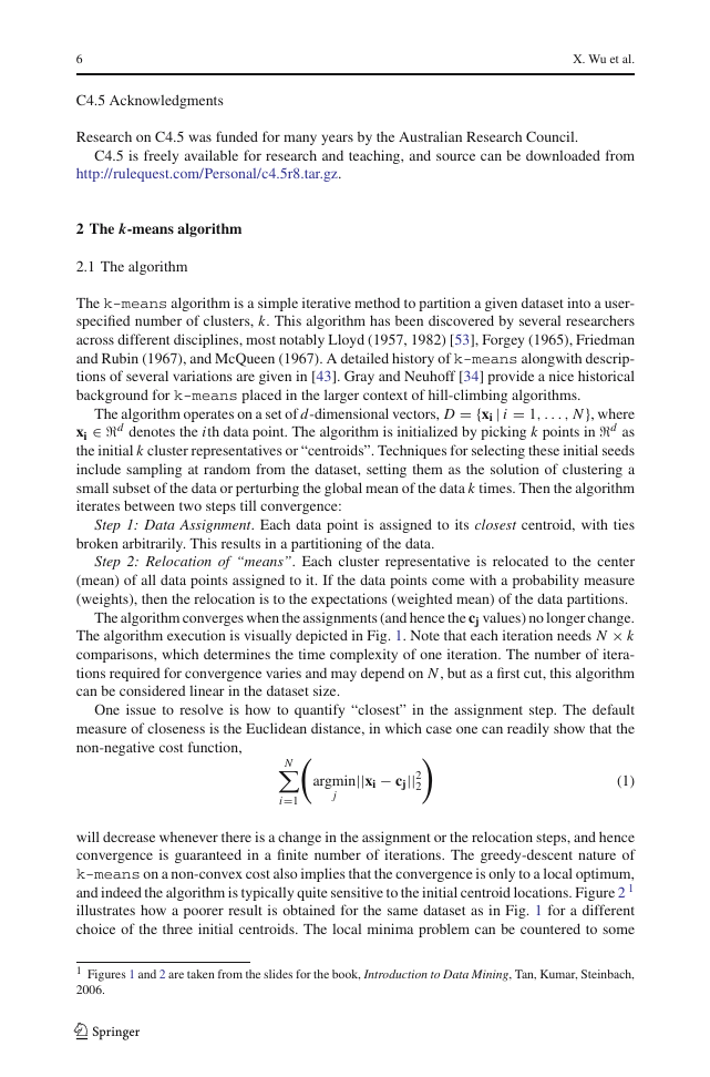
The algorithm execution is visually depicted in Fig. 1. Note that each iteration needs N × k
comparisons, which determines the time complexity of one iteration. The number of itera-
tions required for convergence varies and may depend on N , but as a first cut, this algorithm
can be considered linear in the dataset size.
One issue to resolve is how to quantify “closest” in the assignment step. The default
measure of closeness is the Euclidean distance, in which case one can readily show that the
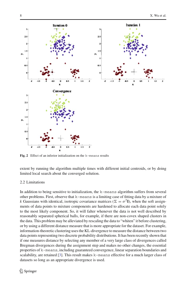
non-negative cost function,
(1)
N
i=1
||xi − cj||2
2
argmin
j
will decrease whenever there is a change in the assignment or the relocation steps, and hence
convergence is guaranteed in a finite number of iterations. The greedy-descent nature of
k-means on a non-convex cost also implies that the convergence is only to a local optimum,
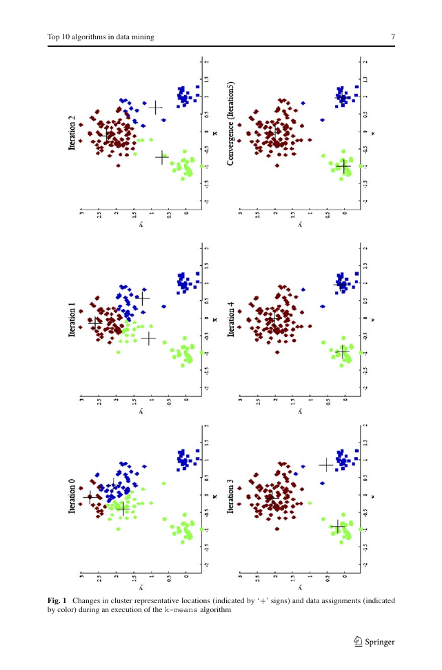
and indeed the algorithm is typically quite sensitive to the initial centroid locations. Figure 2 1
illustrates how a poorer result is obtained for the same dataset as in Fig. 1 for a different
choice of the three initial centroids. The local minima problem can be countered to some
1 Figures 1 and 2 are taken from the slides for the book, Introduction to Data Mining, Tan, Kumar, Steinbach,
2006.
123
�
Top 10 algorithms in data mining
7
Fig. 1 Changes in cluster representative locations (indicated by ‘+’ signs) and data assignments (indicated
by color) during an execution of the k-means algorithm
123
�
8
X. Wu et al.
Fig. 2 Effect of an inferior initialization on the k-means results
extent by running the algorithm multiple times with different initial centroids, or by doing
limited local search about the converged solution.
2.2 Limitations
In addition to being sensitive to initialization, the k-means algorithm suffers from several
other problems. First, observe that k-means is a limiting case of fitting data by a mixture of
k Gaussians with identical, isotropic covariance matrices (� = σ 2I), when the soft assign-
ments of data points to mixture components are hardened to allocate each data point solely
to the most likely component. So, it will falter whenever the data is not well described by
reasonably separated spherical balls, for example, if there are non-covex shaped clusters in
the data. This problem may be alleviated by rescaling the data to “whiten” it before clustering,
or by using a different distance measure that is more appropriate for the dataset. For example,
information-theoretic clustering uses the KL-divergence to measure the distance between two
data points representing two discrete probability distributions. It has been recently shown that
if one measures distance by selecting any member of a very large class of divergences called
Bregman divergences during the assignment step and makes no other changes, the essential
properties of k-means, including guaranteed convergence, linear separation boundaries and
scalability, are retained [3]. This result makes k-means effective for a much larger class of
datasets so long as an appropriate divergence is used.
123
�


 2023年江西萍乡中考道德与法治真题及答案.doc
 2012年重庆南川中考生物真题及答案.doc
 2013年江西师范大学地理学综合及文艺理论基础考研真题.doc
 2020年四川甘孜小升初语文真题及答案I卷.doc
 2020年注册岩土工程师专业基础考试真题及答案.doc
 2023-2024学年福建省厦门市九年级上学期数学月考试题及答案.doc
 2021-2022学年辽宁省沈阳市大东区九年级上学期语文期末试题及答案.doc
 2022-2023学年北京东城区初三第一学期物理期末试卷及答案.doc
 2018上半年江西教师资格初中地理学科知识与教学能力真题及答案.doc
 2012年河北国家公务员申论考试真题及答案-省级.doc
 2020-2021学年江苏省扬州市江都区邵樊片九年级上学期数学第一次质量检测试题及答案.doc
 2022下半年黑龙江教师资格证中学综合素质真题及答案.doc