Algorithms for Reinforcement Learning
Draft of the lecture published in the
Synthesis Lectures on Artificial Intelligence and Machine Learning
series
by
Morgan & Claypool Publishers
Csaba Szepesv´ari
June 9, 2009∗
Contents
1 Overview
2 Markov decision processes
2.1 Preliminaries
. . . . . . . . . . . . . . . . . . . . . . . . . . . . . . . . . . .
2.2 Markov Decision Processes . . . . . . . . . . . . . . . . . . . . . . . . . . . .
2.3 Value functions . . . . . . . . . . . . . . . . . . . . . . . . . . . . . . . . . .
2.4 Dynamic programming algorithms for solving MDPs . . . . . . . . . . . . . .
3 Value prediction problems
3.1 Temporal difference learning in finite state spaces . . . . . . . . . . . . . . .
3.1.1 Tabular TD(0)
. . . . . . . . . . . . . . . . . . . . . . . . . . . . . .
3.1.2 Every-visit Monte-Carlo . . . . . . . . . . . . . . . . . . . . . . . . .
3.1.3 TD(λ): Unifying Monte-Carlo and TD(0) . . . . . . . . . . . . . . . .
. . . . . . . . . . . . . . . . . . . . . . . .
3.2.1 TD(λ) with function approximation . . . . . . . . . . . . . . . . . . .
3.2.2 Gradient temporal difference learning . . . . . . . . . . . . . . . . . .
3.2.3 Least-squares methods . . . . . . . . . . . . . . . . . . . . . . . . . .
3.2 Algorithms for large state spaces
∗Last update: June 25, 2018
1
3
7
7
8
12
16
17
18
18
21
23
25
29
33
36
�
3.2.4 The choice of the function space . . . . . . . . . . . . . . . . . . . . .
42
45
45
47
47
49
50
51
56
56
59
62
64
65
72
72
73
73
73
74
74
78
4 Control
4.1 A catalog of learning problems . . . . . . . . . . . . . . . . . . . . . . . . . .
4.2 Closed-loop interactive learning . . . . . . . . . . . . . . . . . . . . . . . . .
4.2.1 Online learning in bandits . . . . . . . . . . . . . . . . . . . . . . . .
. . . . . . . . . . . . . . . . . . . . . . . .
4.2.2 Active learning in bandits
4.2.3 Active learning in Markov Decision Processes
. . . . . . . . . . . . .
. . . . . . . . . . . . .
4.2.4 Online learning in Markov Decision Processes
4.3 Direct methods . . . . . . . . . . . . . . . . . . . . . . . . . . . . . . . . . .
4.3.1 Q-learning in finite MDPs . . . . . . . . . . . . . . . . . . . . . . . .
4.3.2 Q-learning with function approximation . . . . . . . . . . . . . . . .
. . . . . . . . . . . . . . . . . . . . . . . . . . . . . . .
Implementing a critic . . . . . . . . . . . . . . . . . . . . . . . . . . .
Implementing an actor . . . . . . . . . . . . . . . . . . . . . . . . . .
4.4 Actor-critic methods
4.4.1
4.4.2
5 For further exploration
5.1 Further reading . . . . . . . . . . . . . . . . . . . . . . . . . . . . . . . . . .
5.2 Applications . . . . . . . . . . . . . . . . . . . . . . . . . . . . . . . . . . . .
5.3 Software . . . . . . . . . . . . . . . . . . . . . . . . . . . . . . . . . . . . . .
5.4 Acknowledgements
. . . . . . . . . . . . . . . . . . . . . . . . . . . . . . . .
A The theory of discounted Markovian decision processes
A.1 Contractions and Banach’s fixed-point theorem . . . . . . . . . . . . . . . .
A.2 Application to MDPs . . . . . . . . . . . . . . . . . . . . . . . . . . . . . . .
Abstract
Reinforcement learning is a learning paradigm concerned with learning to control a
system so as to maximize a numerical performance measure that expresses a long-term
objective. What distinguishes reinforcement learning from supervised learning is that
only partial feedback is given to the learner about the learner’s predictions. Further,
the predictions may have long term effects through influencing the future state of the
controlled system. Thus, time plays a special role. The goal in reinforcement learning
is to develop efficient learning algorithms, as well as to understand the algorithms’
merits and limitations. Reinforcement learning is of great interest because of the large
number of practical applications that it can be used to address, ranging from problems
in artificial intelligence to operations research or control engineering. In this book, we
focus on those algorithms of reinforcement learning that build on the powerful theory of
dynamic programming. We give a fairly comprehensive catalog of learning problems,
2
�
Figure 1: The basic reinforcement learning scenario
describe the core ideas together with a large number of state of the art algorithms,
followed by the discussion of their theoretical properties and limitations.
Keywords:
reinforcement learning; Markov Decision Processes; temporal difference learn-
ing; stochastic approximation; two-timescale stochastic approximation; Monte-Carlo meth-
ods; simulation optimization; function approximation; stochastic gradient methods; least-
squares methods; overfitting; bias-variance tradeoff; online learning; active learning; plan-
ning; simulation; PAC-learning; Q-learning; actor-critic methods; policy gradient; natural
gradient
1 Overview
Reinforcement learning (RL) refers to both a learning problem and a subfield of machine
learning. As a learning problem, it refers to learning to control a system so as to maxi-
mize some numerical value which represents a long-term objective. A typical setting where
reinforcement learning operates is shown in Figure 1: A controller receives the controlled
system’s state and a reward associated with the last state transition. It then calculates an
action which is sent back to the system. In response, the system makes a transition to a
new state and the cycle is repeated. The problem is to learn a way of controlling the system
so as to maximize the total reward. The learning problems differ in the details of how the
data is collected and how performance is measured.
In this book, we assume that the system that we wish to control is stochastic. Further,
we assume that the measurements available on the system’s state are detailed enough so
that the the controller can avoid reasoning about how to collect information about the
3
�
state. Problems with these characteristics are best described in the framework of Markovian
Decision Processes (MDPs). The standard approach to ‘solve’ MDPs is to use dynamic
programming, which transforms the problem of finding a good controller into the problem
of finding a good value function. However, apart from the simplest cases when the MDP has
very few states and actions, dynamic programming is infeasible. The RL algorithms that
we discuss here can be thought of as a way of turning the infeasible dynamic programming
methods into practical algorithms so that they can be applied to large-scale problems.
There are two key ideas that allow RL algorithms to achieve this goal. The first idea is to
use samples to compactly represent the dynamics of the control problem. This is important
for two reasons: First, it allows one to deal with learning scenarios when the dynamics is
unknown. Second, even if the dynamics is available, exact reasoning that uses it might
be intractable on its own. The second key idea behind RL algorithms is to use powerful
function approximation methods to compactly represent value functions. The significance
of this is that it allows dealing with large, high-dimensional state- and action-spaces. What
is more, the two ideas fit nicely together: Samples may be focused on a small subset of the
spaces they belong to, which clever function approximation techniques might exploit. It is
the understanding of the interplay between dynamic programming, samples and function
approximation that is at the heart of designing, analyzing and applying RL algorithms.
The purpose of this book is to allow the reader to have a chance to peek into this beautiful
field. However, certainly we are not the first to set out to accomplish this goal. In 1996,
Kaelbling et al. have written a nice, compact survey about the approaches and algorithms
available at the time (Kaelbling et al., 1996). This was followed by the publication of the book
by Bertsekas and Tsitsiklis (1996), which detailed the theoretical foundations. A few years
later Sutton and Barto, the ‘fathers’ of RL, published their book, where they presented their
ideas on RL in a very clear and accessible manner (Sutton and Barto, 1998). A more recent
and comprehensive overview of the tools and techniques of dynamic programming/optimal
control is given in the two-volume book by Bertsekas (2007a,b) which devotes one chapter
to RL methods.1 At times, when a field is rapidly developing, books can get out of date
pretty quickly. In fact, to keep up with the growing body of new results, Bertsekas maintains
an online version of his Chapter 6 of Volume II of his book, which, at the time of writing
this survey counted as much as 160 pages (Bertsekas, 2010). Other recent books on the
subject include the book of Gosavi (2003) who devotes 60 pages to reinforcement learning
algorithms in Chapter 9, concentrating on average cost problems, or that of Cao (2007) who
focuses on policy gradient methods. Powell (2007) presents the algorithms and ideas from an
operations research perspective and emphasizes methods that are capable of handling large
1In this book, RL is called neuro-dynamic programming or approximate dynamic programming. The
term neuro-dynamic programming stems from the fact that, in many cases, RL algorithms are used with
artificial neural networks.
4
�
control spaces, Chang et al. (2008) focuses on adaptive sampling (i.e., simulation-based
performance optimization), while the center of the recent book by Busoniu et al. (2010) is
function approximation.
Thus, by no means do RL researchers lack a good body of literature. However, what seems
to be missing is a self-contained and yet relatively short summary that can help newcomers
to the field to develop a good sense of the state of the art, as well as existing researchers to
broaden their overview of the field, an article, similar to that of Kaelbling et al. (1996), but
with an updated contents. To fill this gap is the very purpose of this short book.
Having the goal of keeping the text short, we had to make a few, hopefully, not too trou-
bling compromises. The first compromise we made was to present results only for the total
expected discounted reward criterion. This choice is motivated by that this is the criterion
that is both widely used and the easiest to deal with mathematically. The next compro-
mise is that the background on MDPs and dynamic programming is kept ultra-compact
(although an appendix is added that explains these basic results). Apart from these, the
book aims to cover a bit of all aspects of RL, up to the level that the reader should be
able to understand the whats and hows, as well as to implement the algorithms presented.
Naturally, we still had to be selective in what we present. Here, the decision was to focus
on the basic algorithms, ideas, as well as the available theory. Special attention was paid to
describing the choices of the user, as well as the tradeoffs that come with these. We tried
to be impartial as much as possible, but some personal bias, as usual, surely remained. The
pseudocode of almost twenty algorithms was included, hoping that this will make it easier
for the practically inclined reader to implement the algorithms described.
The target audience is advanced undergaduate and graduate students, as well as researchers
and practitioners who want to get a good overview of the state of the art in RL quickly.
Researchers who are already working on RL might also enjoy reading about parts of the RL
literature that they are not so familiar with, thus broadening their perspective on RL. The
reader is assumed to be familiar with the basics of linear algebra, calculus, and probability
theory. In particular, we assume that the reader is familiar with the concepts of random
variables, conditional expectations, and Markov chains.
It is helpful, but not necessary,
for the reader to be familiar with statistical learning theory, as the essential concepts will
be explained as needed. In some parts of the book, knowledge of regression techniques of
machine learning will be useful.
This book has three parts. In the first part, in Section 2, we provide the necessary back-
ground.
It is here where the notation is introduced, followed by a short overview of the
theory of Markov Decision Processes and the description of the basic dynamic programming
algorithms. Readers familiar with MDPs and dynamic programming should skim through
this part to familiarize themselves with the notation used. Readers, who are less familiar
5
�
with MDPs, must spend enough time here before moving on because the rest of the book
builds heavily on the results and ideas presented here.
The remaining two parts are devoted to the two basic RL problems (cf. Figure 1), one part
devoted to each.
In Section 3, the problem of learning to predict values associated with
states is studied. We start by explaining the basic ideas for the so-called tabular case when
the MDP is small enough so that one can store one value per state in an array allocated in
a computer’s main memory. The first algorithm explained is TD(λ), which can be viewed
as the learning analogue to value iteration from dynamic programming. After this, we
consider the more challenging situation when there are more states than what fits into a
computer’s memory. Clearly, in this case, one must compress the table representing the
values. Abstractly, this can be done by relying on an appropriate function approximation
method. First, we describe how TD(λ) can be used in this situation. This is followed by the
description of some new gradient based methods (GTD2 and TDC), which can be viewed
as improved versions of TD(λ) in that they avoid some of the convergence difficulties that
TD(λ) faces. We then discuss least-squares methods (in particular, LSTD(λ) and λ-LSPE)
and compare them to the incremental methods described earlier. Finally, we describe choices
available for implementing function approximation and the tradeoffs that these choices come
with.
The second part (Section 4) is devoted to algorithms that are developed for control learning.
First, we describe methods whose goal is optimizing online performance.
In particular,
we describe the “optimism in the face of uncertainty” principle and methods that explore
their environment based on this principle. State of the art algorithms are given both for
bandit problems and MDPs. The message here is that clever exploration methods make
a large difference, but more work is needed to scale up the available methods to large
problems. The rest of this section is devoted to methods that aim at developing methods
that can be used in large-scale applications. As learning in large-scale MDPs is significantly
more difficult than learning when the MDP is small, the goal of learning is relaxed to
learning a good enough policy in the limit. First, direct methods are discussed which aim at
estimating the optimal action-values directly. These can be viewed as the learning analogue
of value iteration of dynamic programming. This is followed by the description of actor-
critic methods, which can be thought of as the counterpart of the policy iteration algorithm
of dynamic programming. Both methods based on direct policy improvement and policy
gradient (i.e., which use parametric policy classes) are presented.
The book is concluded in Section 5, which lists some topics for further exploration.
6
�
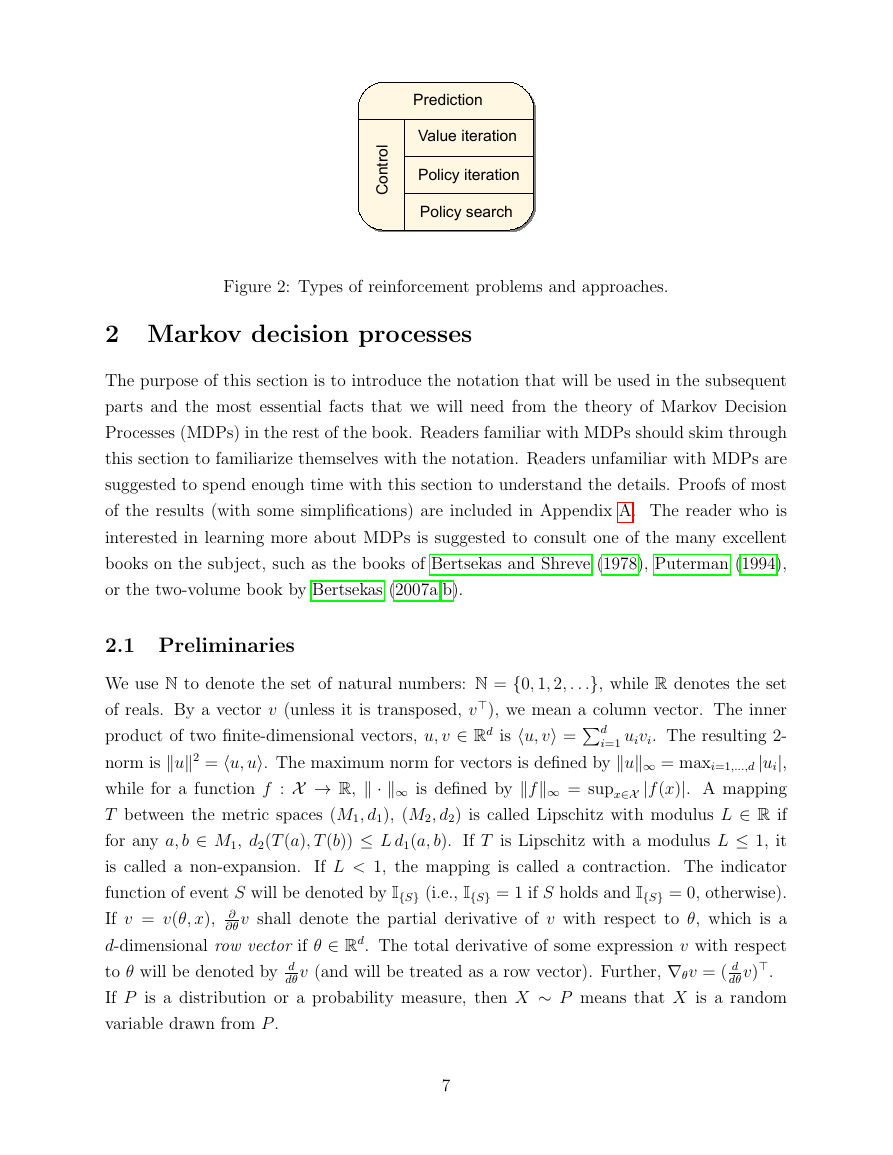
Figure 2: Types of reinforcement problems and approaches.
2 Markov decision processes
The purpose of this section is to introduce the notation that will be used in the subsequent
parts and the most essential facts that we will need from the theory of Markov Decision
Processes (MDPs) in the rest of the book. Readers familiar with MDPs should skim through
this section to familiarize themselves with the notation. Readers unfamiliar with MDPs are
suggested to spend enough time with this section to understand the details. Proofs of most
of the results (with some simplifications) are included in Appendix A. The reader who is
interested in learning more about MDPs is suggested to consult one of the many excellent
books on the subject, such as the books of Bertsekas and Shreve (1978), Puterman (1994),
or the two-volume book by Bertsekas (2007a,b).
product of two finite-dimensional vectors, u, v ∈ Rd is u, v =d
2.1 Preliminaries
We use N to denote the set of natural numbers: N = {0, 1, 2, . . .}, while R denotes the set
of reals. By a vector v (unless it is transposed, v), we mean a column vector. The inner
i=1 uivi. The resulting 2-
norm is u2 = u, u. The maximum norm for vectors is defined by u∞ = maxi=1,...,d |ui|,
while for a function f : X → R, · ∞ is defined by f∞ = supx∈X |f (x)|. A mapping
T between the metric spaces (M1, d1), (M2, d2) is called Lipschitz with modulus L ∈ R if
for any a, b ∈ M1, d2(T (a), T (b)) ≤ L d1(a, b). If T is Lipschitz with a modulus L ≤ 1, it
is called a non-expansion.
If L < 1, the mapping is called a contraction. The indicator
function of event S will be denoted by I{S} (i.e., I{S} = 1 if S holds and I{S} = 0, otherwise).
∂
∂θ v shall denote the partial derivative of v with respect to θ, which is a
If v = v(θ, x),
d-dimensional row vector if θ ∈ Rd. The total derivative of some expression v with respect
dθ v).
to θ will be denoted by d
If P is a distribution or a probability measure, then X ∼ P means that X is a random
variable drawn from P .
dθ v (and will be treated as a row vector). Further, ∇θv = ( d
7
!"#$%&'%()*+,-#.%'#"+'%()!(,%&/.%'#"+'%()!(,%&/.0#+"&12()'"(,�
2.2 Markov Decision Processes
For ease of exposition, we restrict our attention to countable MDPs and the discounted total
expected reward criterion. However, under some technical conditions, the results extend to
continuous state-action MDPs, too. This also holds true for the results presented in later
parts of this book.
A countable MDP is defined as a triplet M = (X ,A,P0), where X is the countable non-
empty set of states, A is the countable non-empty set of actions. The transition probability
kernel P0 assigns to each state-action pair (x, a) ∈ X ×A a probability measure over X × R,
which we shall denote by P0(·|x, a). The semantics of P0 is the following: For U ⊂ X × R,
P0(U|x, a) gives the probability that the next state and the associated reward belongs to the
set U provided that the current state is x and the action taken is a.2 We also fix a discount
factor 0 ≤ γ ≤ 1 whose role will become clear soon.
The transition probability kernel gives rise to the state transition probability kernel, P, which,
for any (x, a, y) ∈ X × A × X triplet gives the probability of moving from state x to some
other state y provided that action a was chosen in state x:
P(x, a, y) = P0({y} × R| x, a).
In addition to P, P0 also gives rise to the immediate reward function r : X × A → R,
which gives the expected immediate reward received when action a is chosen in state x: If
(Y(x,a), R(x,a)) ∼ P0(·| x, a), then
r(x, a) = ER(x,a)
.
In what follows, we shall assume that the rewards are bounded by some quantity R > 0:
for any (x, a) ∈ X × A, |R(x,a)| ≤ R almost surely.3
It is immediate that if the random
rewards are bounded by R then r∞ = sup(x,a)∈X×A |r(x, a)| ≤ R also holds. An MDP is
called finite if both X and A are finite.
Markov Decision Processes are a tool for modeling sequential decision-making problems
where a decision maker interacts with a system in a sequential fashion. Given an MDP M,
this interaction happens as follows: Let t ∈ N denote the current time (or stage), let Xt ∈ X
2The probability P0(U|x, a) is defined only when U is a Borel-measurable set. Borel-measurability is a
technical notion whose purpose is to prevent some pathologies. The collection of Borel-measurable subsets
of X × R include practically all “interesting” subsets X × R. In particular, they include subsets of the form
{x} × [a, b] and subsets which can be obtained from such subsets by taking their complement, or the union
(intersection) of at most countable collections of such sets in a recursive fashion.
3“Almost surely” means the same as “with probability one” and is used to refer to the fact that the
statement concerned holds everywhere on the probability space with the exception of a set of events with
measure zero.
8
�



 2023年江西萍乡中考道德与法治真题及答案.doc
 2012年重庆南川中考生物真题及答案.doc
 2013年江西师范大学地理学综合及文艺理论基础考研真题.doc
 2020年四川甘孜小升初语文真题及答案I卷.doc
 2020年注册岩土工程师专业基础考试真题及答案.doc
 2023-2024学年福建省厦门市九年级上学期数学月考试题及答案.doc
 2021-2022学年辽宁省沈阳市大东区九年级上学期语文期末试题及答案.doc
 2022-2023学年北京东城区初三第一学期物理期末试卷及答案.doc
 2018上半年江西教师资格初中地理学科知识与教学能力真题及答案.doc
 2012年河北国家公务员申论考试真题及答案-省级.doc
 2020-2021学年江苏省扬州市江都区邵樊片九年级上学期数学第一次质量检测试题及答案.doc
 2022下半年黑龙江教师资格证中学综合素质真题及答案.doc