American Journal of Computational Mathematics, 2017, 7, 350-370
http://www.scirp.org/journal/ajcm
ISSN Online: 2161-1211
ISSN Print: 2161-1203
Numerical Simulation of Groundwater
Pollution Problems Based on Convection
Diffusion Equation
Lingyu Li, Zhe Yin*
College of Mathematics and Statistics, Shandong Normal University, Jinan, China
How to cite this paper: Li, L.Y. and Yin, Z.
(2017) Numerical Simulation of Groundwa-
ter Pollution Problems Based on Convection
Diffusion Equation. American Journal of
Computational Mathematics, 7, 350-370.
https://doi.org/10.4236/ajcm.2017.73025
Received: August 2, 2017
Accepted: September 3, 2017
Published: September 6, 2017
Copyright © 2017 by authors and
Scientific Research Publishing Inc.
This work is licensed under the Creative
Commons Attribution International
License (CC BY 4.0).
http://creativecommons.org/licenses/by/4.0/
Open Access
Abstract
The analytical solution of the convection diffusion equation is considered by
two-dimensional Fourier transform and the inverse Fourier transform. To get
the numerical solution, the Crank-Nicolson finite difference method is con-
structed, which is second-order accurate in time and space. Numerical simu-
lation shows excellent agreement with the analytical solution. The dynamic
visualization of the simulating results is realized on ArcGIS platform. This
work provides a quick and intuitive decision-making basis for water resources
protection, especially in dealing with water pollution emergencies.
Keywords
Groundwater Pollution, Two-Dimensional Convection Diffusion Equation,
Finite Difference Method, Visualization, Numerical Simulation
1. Introduction
Numerical simulations of groundwater pollution problems have been given
increased emphasis in recent years. Groundwater is often contaminated by, for
example, the sewage out of factories or mines and the chemical fertilizer and
pesticide in agriculture, in particular, nitrate pollution of groundwater in rivers
basins and agricultural watersheds are going from bad to worse all over the
world [1]. Groundwater protection is an issue with both social and economic
significant (e.g., Chen et al. [2]), so to simulate the movement of the contaminated
groundwater, lots of mathematical models have been applied extensively and the
use of numerical simulations seems to be inevitable.
Generally, analytical solutions can not be derived for most classical models,
DOI: 10.4236/ajcm.2017.73025 Sep. 6, 2017
350
American Journal of Computational Mathematics
�
L. Y. Li, Z. Yin
consequently, the development of numerical solutions is required. S. Hasnain
and M. Saqib originate results with finite difference schemes to approximate the
solution of the classical Fisher Kolmogorov Petrovsky Piscounov (KPP) equation
from population dynamics, their results show that Crank-Nicolson is very
efficient and reliably numerical scheme for solving one-dimension fishers KPP
equation [3]. During the last three decades, numerous transport problems have
been solved numerical [4], theoretical numerical models are necessary tools were
presented [5], the technique of intimating the movement of groundwater flow is
improved greatly, see [6] [7] [8] and the references therein. Dillon gave many
mathematical models and numerical methods for solving the groundwater
problems [6]. Li and Jiao derived the analytical solutions of tidal groundwater
flow in coastal two-aquifer system [7]. Sun applied a sort of numerical methods
to simulate the movement of contaminants in groundwater [8].
At present, the researches on groundwater pollution problems are mainly
divided into two categories at home and abroad [9] [10]. On one hand, people
generally study various discrete numerical schemes of mathematical models (i.e.
the corresponding partial differential equations) for groundwater pollution, by
doing lots of related works, the numerical solution is obtained and the
convergence is analyzed, Lin, L. et al. [9] derived a simplified numerical model
of groundwater and solute transport. On the other hand, people develop the
simulation software of groundwater numerical [11] [12] [13], particularly,
numerical simulation software of groundwater system has been developed,
which is widely used because of its modularity, visualization, interaction and
diversification, such as, the popular GIS, which is used to provide the visualization
methods and approaches of groundwater pollution diffusion simulation. Qin, R.
et al. [11] presented a GIS-based software for forecasting pollutant drift on
coastal water surfaces using fractional Brownian motion, it can be used to study
on red tide drift. Valocchi, A. J. et al. [12] developed a series of interactive web
simulation models to help students understand the coupled physical, chemical,
and microbiological processes that affect the transport and fate of pollutants in
groundwater. Li, J. et al. [13] mentioned that HYDRUS-1D software can
simulate different concentrations of pollutants reaching the shallow aquifer
under some vadose zone conditions, he presented a method for quantitative
groundwater pollution assessment based on grey relational analysis (GRA).
A lot of research literatures about the former have been represented in China.
In recent years, with the wide application of new technology and new method,
many scholars have made innovations in theory and methodology, by means of
the combination of theory and research direction of numerical model theory,
they combine the theory of numerical model with the related acknowledges, so
as to improve the reliability of simulation results [10]. However, most of the
previous literatures only simulate the surface water. By studying the literature
[11] [12] [13], we found that the visual simulation of the actual problems of
groundwater pollution is rare. If the above two were combined, it will not only
351
American Journal of Computational Mathematics
DOI: 10.4236/ajcm.2017.73025
�
L. Y. Li, Z. Yin
in theory and application of important values, but also innovative, advanced and
applied.
In book [14], Kovarik, K. sets his sights on reviewing the whole group of
numerical methods from the oldest (the finite differences method), and discusses
the basic equations of a groundwater flow and of the transport of pollutants in a
porous medium. Therefore, we would like to use the finite difference method to
study the numerical simulation methods about mathematical models with seepage
of groundwater pollution. In order to improve the accuracy in the temporal
direction, we propose a second-order scheme which based on centered Crank-
Nicolson finite difference scheme [15]-[20]. And we simulate the water pollution
problems in a certain area and verify the validity and practicability of the model
and its algorithm. Meanwhile, the dynamic visualization of simulation results is
realized on ArcGIS platform. We hope that our work can provide an important
basis for water pollution accident emergency response and decision-making, and
can be used for environmental protection personnel to deal with water pollution
emergencies.
The paper is organized as follows. In Section 2, we give the analytical solution
of the Equations (1)-(5) by two-dimensional Fourier transform and the inverse
Fourier transform. In Section 3, we introduce some notations, present the
Crank-Nicolson finite difference discretization of the governing equation and derive
the truncation error. Numerical experiment is given, exact solution comparisons
with numerical solution are also discussed in Section 4. Visualization of simulation
results based on GIS (ArcGIS figures) is presented in Section 5. Finally,
conclusions and suggestions are drawn in Section 6.
2. Analytical Solution
In this paper, we consider the following physical problem. The leakage of the
sewage pool in a paper mill causes the seepage of sewage, and the concentration
of some substance in any point in the underground water is a function of space
coordinate and time, i.e.
. We take an micro-body in the underground
water, the concentration change of it is caused by two aspects: One is diffusion,
including molecular diffusion and osmotic dispersion, another is the mass flux
caused by the average liquid motion. In this problem, we assume that the
seepage area is an infinite plane, and the groundwater flow is a one-dimensional
one, the diffusion of pollutants is a two-dimensional dispersion, and the medium
is a porous medium.
C x y t
,
(
)
,
We take O as the coordinate origin (pollution source), take the infinite plane
as the plane O-xy, the flow direction and the x axis direction are consistent.
Then, our problem can be illustrated by the following two-dimensional parabolic
equation with convection term
C
∂
t
∂
=
D
x
D
2
+
C
∂
2
x
∂
C x y
(
,
y
,0
2
C
∂
2
y
∂
)
=
0,
−
v
,
C
∂
x
∂
(
x y
,
(
0
< < +∞ >
x
t
,
)
0 ,
(1)
)
≠
(
)
0,0 ,
(2)
DOI: 10.4236/ajcm.2017.73025
352
American Journal of Computational Mathematics
�
+∞ +∞
∫
,
d d
∫
−∞ −∞
(
C x y t
,
(
C x y t
,
nC x y m
,
)
)
=
(
(
0,
0,
=
=
>
>
t
t
,
lim
x
→±∞
lim
y
→±∞
L. Y. Li, Z. Yin
)
0 ,
)
0 .
(3)
(4)
(5)
xD and
Problem (1)-(5) arises in the mathematical modeling of transport processes
that exhibit diffusion, in which, the unknown C stands for the concentration of a
yD are the
solute, x and y are the horizontal coordinates, t is the time,
xD
longitudinal and transversal dispersion coefficients respectively (namely,
yD are the aquifer transmissivity, subscripts x and y indicate the respective
and
directions). m is the instantaneous injected solute mass per unit length of porous
medium, v is the mean pore velocity, and n indicates the effective porosity. At
the initial stage, we suppose, there is no contaminant in the river, and when
t ≥ the concentration at
0
There are different approaches to solve two-dimensional parabolic equation, a
series of analytical solutions derived from the basic physical principles have been
presented which are mostly suitable under special boundary conditions [21]. In
this part, we give the analytical solution of the Equations (1)-(5) by using
two-dimensional Fourier transform and the inverse Fourier transform.
x = remains at
C C=
0
0
.
First of all, we give the definition of the two-dimensional Fourier transform
and the inverse Fourier transform and some properties to be used in the
following. The Fourier transform of
(
f x y
,
)
2π
−
x y
d d ,
(
i x
(6)
(
ξ ξ
1
2
=
ˆ
f
(
)
)
,
2
∫∫
R
+
ξ ξ
1
2
(
f x y is written to
,
)
)
exp
⋅
)
d d ,
ξ ξ ξ ξ
1
2
(
f x y as follows
y
(
i x
+
(
y
)
,
2
1
the definition of the inverse Fourier transform for
(
f x y
,
)
and the derivative properties of the Fourier transform are
exp 2π
(
ξ ξ
1
2
∫∫
=
ˆ
f
)
)
,
⋅
R
2
(7)
f
∂
=
∂
x
∂
x
∂
=
f
2
(
2
i
2π
ξ
1
ˆ
f
,
i
2π
2
)
2
ξ
1
ˆ
f
,
=
f
∂
y
∂
∂
y
∂
f
2
2
i
2π
ξ
2
ˆ
f
,
=
(
i
2π
2
)
2
ξ
2
ˆ
f
.
We do Fourier transformation of x and y (this transformation has no effect on
the independent variables, so there is no Fourier transformation for t, so it has
nothing to do with the t to the Equation (1) firstly.
ˆ
C
∂
t
∂
= −
4π
2
ˆ
D C
2
ξ
x
1
−
2
4π
ˆ
D C
2
ξ
y
2
−
2
2π
ˆ
iv C
ξ
1
,
deal with the conditional Eqution (3), we have
.m
n
C x y
d d
+∞ +∞
−∞ −∞
=
∫
∫
(8)
(9)
Then, we do the Fourier transformation to the initial condition Eqution (2),
by Eqution (9), we have
353
American Journal of Computational Mathematics
DOI: 10.4236/ajcm.2017.73025
�
L. Y. Li, Z. Yin
ˆ
C
(
ξ ξ
1
2
,
,0
)
=
∫∫
R
2
(
δ
x y
,
)
⋅
exp
(
m
n
2π
−
(
i x
ξ ξ
1
2
+
y
)
)
x y
d d ,
in which
(
δ
x y
,
)
(
,
∞
=
0,
(
)
=
)
x y
,
0,0
other points
,
δ+∞ +∞
(
∫
−∞ −∞
∫
x y
,
)
x y
d d
=
1,
(10)
(11)
it is called the Dirac function, also called the generalized function. We denote
(
g x y
,
)
=
(
δ
x y
,
)
⋅
exp
(
it can be easily to proved
2π
−
(
i x
ξ ξ
2
+
y
1
)
)
,
(12)
⋅
g
(
)0,0
=
m
n
m
n
.
Notice Eqution (8) is a separable equation, so we have
)
(
= −
2
D
ξ
x
1
iv
ξ
1
2
ξ
y
2
4π
4π
2π
D
+
−
(
)
2
2
ˆd
C
ˆ
C
t
d ,
integrate the both sides of the Eqution (14) about variable t, we have
ln
ˆ
C
(
= −
(
2
4π
2
D
ξ
x
1
+
2
4π
D
2
ξ
y
2
)
−
2π
iv
ξ
1
)
t C
+
0
.
0C is a constant and it has nothing with other variables (the same
where
below).
So, we get the general solution of Eqution (8)
)
substitute 0 for t in formula (16), using Eqution (10), we obtain
ˆ
C C
0
2
D
ξ
x
1
iv
ξ
1
exp
2
ξ
y
2
4π
4π
2π
D
(
(
)
=
−
+
−
(
)
t
,
⋅
2
2
ˆ
C
(
)
ξ ξ =
1
,0
,
2
C
0
⋅
( )
exp 0
=
m
n
,
C
0
=
m
n
,
in fact, by Equtions ((16) and (17)) we have the solution of Eqution (8)
(13)
(14)
(15)
(16)
(17)
(18)
t
.
2
2
2
⋅
y
)
)
(
+
−
−
+
−
)
(
(
D
2π
4π
4π
2
ξ
y
2
exp
(
(
(
i x
iv
ξ
1
d d
1
2
D
ξ
x
1
exp 2π
mC
ˆ
=
n
ξ ξ ξ ξ
1
2
)
⋅
(
4π
−
)
Next, for Eqution (16), we do the inverse Fourier transform
,
(
(
4π
−
(
ξ ξ
1
2
)
y
)
d d
1
)
)
2π
−
iy
ξ ξ ξ
2
2
2
ξ
y
2
)
4π
)
ξ ξ
1
2
exp 2π
d d
ξ ξ
1
2
2
D t
ξ
x
1
i
2π
ξ
1
2
D
ξ
x
1
2
D
ξ
x
1
(
i x
(
i x
D t
y
D t
x
2
ξ
y
2
4π
2π
2π
2π
2π
ξ
1
D
D
vt
vt
)
)
+
−
+
+
+
+
−
+
−
+
−
)
)
)
)
2
)
t
⋅
x
−
+
+
(
(
(
y
x
)
(
)
2
2
2
iy
ξ ξ ξ
2
2
d d
1
d d
ξ ξ
1
2
t
2π
iv
ξ
1
iv
ξ
1
)
(
i
2π
ξ
1
)
ξ
2
−
2
2
2π
2
−
2π
2
D t
ξ
x
2
(
(
i x
2
vt
−
D t
x
)
−
2π
D t
x
ξ
1
−
C x y t
,
,
(
)
=
=
=
=
=
=
ˆ
C
2
(
ξ ξ
1
2
,
t
∫∫
R
m
n
m
n
m
n
m
n
∫∫
R
∫∫
R
∫∫
R
∫∫
R
2
2
2
2
m
n
∫∫
R
2
(
exp
exp
exp
(
(
exp
exp
(
D t
y
ξ
2
−
iy
D t
y
2
2
−
vt
x
−
D t
4
x
2
)
−
2
y
D t
y
4
d d
ξ ξ
1
2
DOI: 10.4236/ajcm.2017.73025
354
American Journal of Computational Mathematics
�
L. Y. Li, Z. Yin
=
m
n
⋅
exp
(
−
2
)
vt
x
−
D t
4
x
−
2
y
D t
y
4
⋅
+∞
−∞
∫
exp
−
2π
D t
x
ξ
1
−
(
i x
2
vt
−
D t
x
) 2
d
ξ
1
⋅
∫
+∞
−∞
exp
−
2π
D t
y
ξ
2
−
iy
D t
y
2
2
d .
ξ
2
(19)
And because
exp
(
t−
+∞
∫
−∞
)2
exp
is an even function, it is obviously to get
(
exp
π,
t
−
t
−
=
d
t
d
t
=
2
)
(
)
+∞
2
2
∫
0
(20)
therefore, take Equation (19) into account, we have
+∞
−∞
∫
exp
−
2π
D t
x
ξ
1
−
)
(
i x
2
vt
−
D t
x
2
d
ξ
1
(
i x
2
vt
−
D t
x
=
=
2π
2π
1
D t
x
1
D t
x
+∞
−∞
∫
+∞
−∞
∫
exp
exp
−
−
where
(
i x
2π
written to
)
vt
−
D t
x
2π
D t
x
ξ
1
−
2π
D t
x
ξ
1
−
(
i x
2
vt
−
D t
x
)
)
2
2
(
d 2π
D t
x
ξ
1
)
(21)
d 2π
D t
x
ξ
1
−
)
(
i x
2
vt
−
D t
x
,
is a constant, using Equaiton (20), then Equaiton (21) can be
+∞
−∞
∫
exp
−
2π
D t
x
ξ
1
−
(
i x
2
vt
−
D t
x
) 2
d
ξ
1
=
2π
π
D t
x
=
1
2 π
D t
x
,
(22)
similarly, we have
+∞
−∞
∫
exp
−
2π
D t
y
ξ
2
−
iy
D t
y
2
2
d
ξ
2
=
1
2 π
D t
y
.
(23)
If we plug Equation (19) and Equation (22) back into Equation (23), we obtain
C x y t
,
,
(
)
=
=
m
n
m
n
⋅
⋅
1
2 π
D t
x
1
4π
t D D
x
1
⋅
2 π
⋅
exp
y
it follows from the above equations that
D t
y
(
−
⋅
exp
)
vt
x
−
D t
4
x
2
(
−
2
)
vt
x
−
D t
4
x
−
2
y
D t
y
4
−
2
y
D t
y
4
,
(24)
C x y t
,
,
(
)
=
m
n
4π
t D D
x
⋅
exp
y
(
−
)2
vt
x
−
D t
4
x
−
2
y
D t
y
4
.
(25)
DOI: 10.4236/ajcm.2017.73025
As mentioned above, for Equation (19), taking two-dimensional Fourier
transform and the inverse Fourier transform of both sides, its analytical solution
355
American Journal of Computational Mathematics
�
L. Y. Li, Z. Yin
m
n
4π
t D D
x
⋅
exp
y
(
−
)2
vt
x
−
D t
4
x
−
2
y
D t
y
4
.
(26)
C x y t
,
,
(
)
=
is obtained.
Using MATLAB software to program, under the condition of
L
x
L=
y
=
0 :30
,
1T = or
5T = ,
5m
= ,
n
v =
0.1
, we give the figures of analytical solution
when the diffusion coefficient is
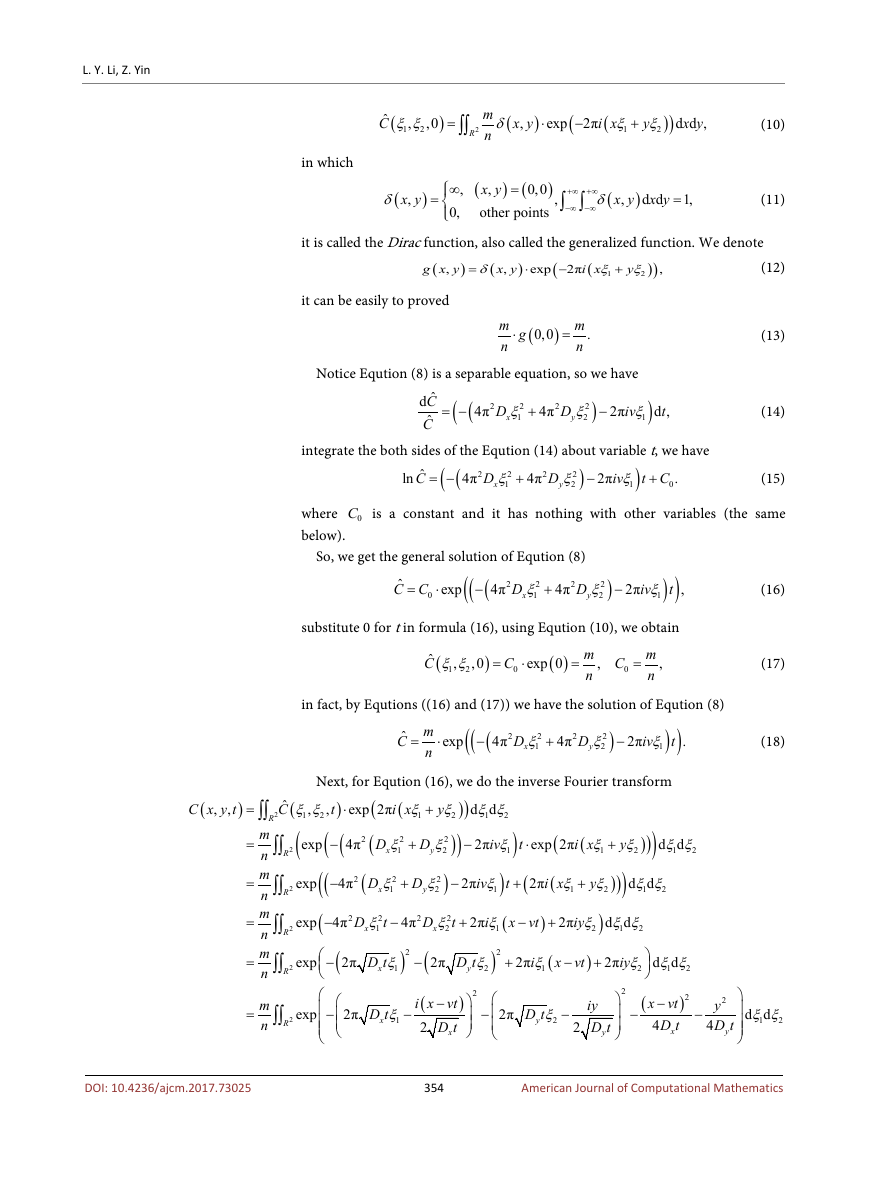
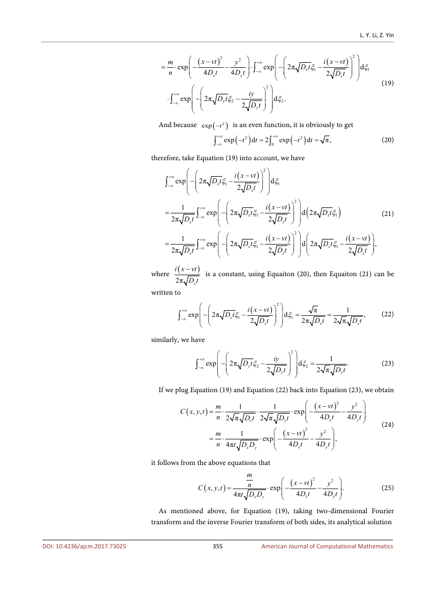
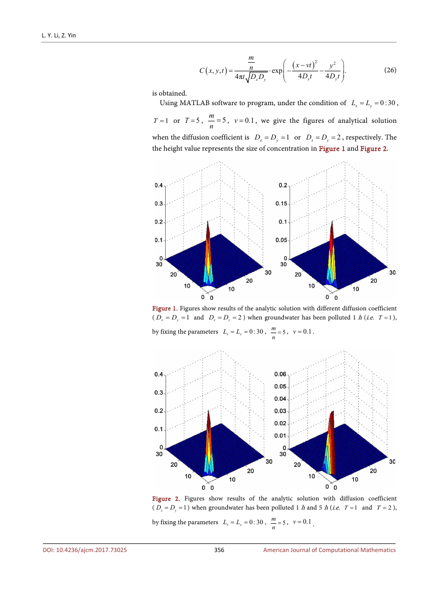
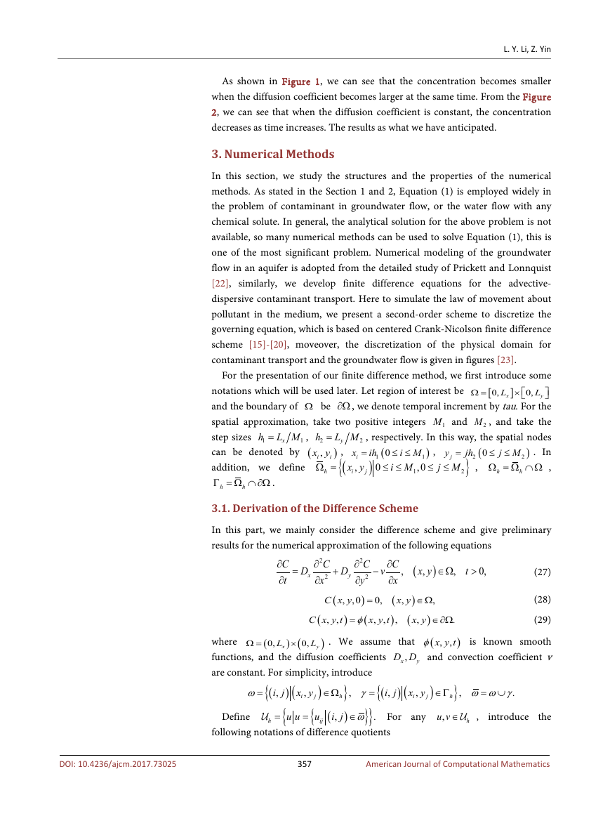
= , respectively. The
the height value represents the size of concentration in Figure 1 and Figure 2.
= or
1
D D=
D D=
2
x
y
x
y
Figure 1. Figures show results of the analytic solution with different diffusion coefficient
D
(
1T = ),
x
= ) when groundwater has been polluted 1 h (i.e.
= and
D D=
D=
1
2
y
x
y
by fixing the parameters
L
x
L=
y
=
0 : 30
,
5m
= ,
n
v =
0.1
.
Figure 2. Figures show results of the analytic solution with diffusion coefficient
D D=
(
T = ),
1
= ) when groundwater has been polluted 1 h and 5 h (i.e.
1T = and
2
x
y
DOI: 10.4236/ajcm.2017.73025
by fixing the parameters
L
x
L=
y
=
0 : 30
,
5m
= ,
n
v =
0.1
.
356
American Journal of Computational Mathematics
�
L. Y. Li, Z. Yin
As shown in Figure 1, we can see that the concentration becomes smaller
when the diffusion coefficient becomes larger at the same time. From the Figure
2, we can see that when the diffusion coefficient is constant, the concentration
decreases as time increases. The results as what we have anticipated.
3. Numerical Methods
In this section, we study the structures and the properties of the numerical
methods. As stated in the Section 1 and 2, Equation (1) is employed widely in
the problem of contaminant in groundwater flow, or the water flow with any
chemical solute. In general, the analytical solution for the above problem is not
available, so many numerical methods can be used to solve Equation (1), this is
one of the most significant problem. Numerical modeling of the groundwater
flow in an aquifer is adopted from the detailed study of Prickett and Lonnquist
[22], similarly, we develop finite difference equations for the advective-
dispersive contaminant transport. Here to simulate the law of movement about
pollutant in the medium, we present a second-order scheme to discretize the
governing equation, which is based on centered Crank-Nicolson finite difference
scheme [15]-[20], moveover, the discretization of the physical domain for
contaminant transport and the groundwater flow is given in figures [23].
For the presentation of our finite difference method, we first introduce some
notations which will be used later. Let region of interest be
and the boundary of Ω be ∂Ω , we denote temporal increment by tau. For the
2M , and take the
spatial approximation, take two positive integers
L M
h
step sizes
, respectively. In this way, the spatial nodes
,
=
y
2
2
can be denoted by (
)
(
. In
,
ih
ix
x y
0
,i
=
≤ ≤
i
{
1
(
)
x y
,
0
≤ ≤
Ω =
addition, we define
Ω = Ω ∩ Ω ,
i
Γ = Ω ∩ ∂Ω .
h
)
,
jy
=
j M
≤ ≤
(
jh
0
}
2
,
i M
1
,0
≤ ≤
i M
1M and
L M
x
j M
L
0,
Ω =
×
h
1
L
x
0,
=
)
[
]
h
1
2
1
h
h
h
2
y
j
3.1. Derivation of the Difference Scheme
In this part, we mainly consider the difference scheme and give preliminary
results for the numerical approximation of the following equations
C
∂
t
∂
=
D
x
2
C
∂
2
x
∂
+
D
y
−
v
0,
2
C
∂
2
y
∂
)
,0
=
(
φ=
x y t
,
,
,
C
∂
x
∂
(
x y
,
(
)
,
(
C x y t
,
C x y
,
)
(
,
(
x y
,
)
,
∈Ω
t
>
0,
(27)
)
∈ Ω (28)
,
)
∈ ∂Ω (29)
x y
,
(
is known smooth
x y t
,
,
φ
D D and convection coefficient v
,x
)
.
y
. We assume that
)
(
y
)
(
×
L
0,
0,
L
x
Ω =
where
functions, and the diffusion coefficients
are constant. For simplicity, introduce
}
{
(
γ
=
}
}
)
j ω
)
x y
i
{
u
ij
) (
j
{
u u
{
(
Define
∈Ω
ω
=
∈
=
=
(
i
i
i
,
.
,
,
,
h
h
j
following notations of difference quotients
) (
j
x y
,
i
j
)
∈Γ
}
,
h
= ∪
.
ω ω γ
,
For any
u v ∈ ,
,
h
introduce
the
DOI: 10.4236/ajcm.2017.73025
357
American Journal of Computational Mathematics
�


 2023年江西萍乡中考道德与法治真题及答案.doc
 2012年重庆南川中考生物真题及答案.doc
 2013年江西师范大学地理学综合及文艺理论基础考研真题.doc
 2020年四川甘孜小升初语文真题及答案I卷.doc
 2020年注册岩土工程师专业基础考试真题及答案.doc
 2023-2024学年福建省厦门市九年级上学期数学月考试题及答案.doc
 2021-2022学年辽宁省沈阳市大东区九年级上学期语文期末试题及答案.doc
 2022-2023学年北京东城区初三第一学期物理期末试卷及答案.doc
 2018上半年江西教师资格初中地理学科知识与教学能力真题及答案.doc
 2012年河北国家公务员申论考试真题及答案-省级.doc
 2020-2021学年江苏省扬州市江都区邵樊片九年级上学期数学第一次质量检测试题及答案.doc
 2022下半年黑龙江教师资格证中学综合素质真题及答案.doc