Research Collection
Journal Article
Iterated extended Kalman filter based visual-inertial odometry
using direct photometric feedback
Author(s):
Bloesch, Michael; Burri, Michael; Omari, Sammy; Hutter, Marco; Siegwart, Roland
Publication Date:
2017-09
Permanent Link:
https://doi.org/10.3929/ethz-b-000187364
Originally published in:
The International Journal of Robotics Research 36(10), http://doi.org/10.1177/0278364917728574
Rights / License:
In Copyright - Non-Commercial Use Permitted
This page was generated automatically upon download from the ETH Zurich Research Collection. For more
information please consult the Terms of use.
ETH Library
�
IEKF-based Visual-Inertial Odometry
using Direct Photometric Feedback
Journal Title
XX(X):1–18
cThe Author(s) 2017
Reprints and permission:
sagepub.co.uk/journalsPermissions.nav
DOI: 10.1177/ToBeAssigned
www.sagepub.com/
Michael Bloesch1, Michael Burri1, Sammy Omari1, Marco Hutter1, Roland Siegwart1
Abstract
This paper presents a visual-inertial odometry framework which tightly fuses inertial measurements with visual data
from one or more cameras, by means of an iterated extended Kalman filter (IEKF). By employing image patches as
landmark descriptors, a photometric error is derived, which is directly integrated as an innovation term in the filter
update step. Consequently, the data association is an inherent part of the estimation process and no additional feature
extraction or matching processes are required. Furthermore, it enables the tracking of non-corner shaped features,
such as lines, and thereby increases the set of possible landmarks. The filter state is formulated in a fully robocentric
fashion, which reduces errors related to nonlinearities. This also includes partitioning of a landmark’s location estimate
into a bearing vector and distance and thereby allows an undelayed initialization of landmarks. Overall, this results
in a compact approach which exhibits a high level of robustness with respect to low scene texture and motion blur.
Furthermore, there is no time-consuming initialization procedure and pose estimates are available starting at the
second image frame. We test the filter on different real datasets and compare it to other state-of-the-art visual-inertial
frameworks. The experimental results show that robust localization with high accuracy can be achieved with this filter-
based framework.
Keywords
Visual-Inertial Odometry,
Cameras
Iterated Extended Kalman Filter, Photometric Error, Tight
Information Fusion, Multiple
1 Introduction
Robust and high-bandwidth estimation of ego-motion is a
key factor to enable the operation of autonomous robots.
For dynamically controlled robots, such as aerial vehicles or
legged robots, a reliable state estimate is essential: Failures
of the state estimator can quickly lead to damage of the
hardware and its surroundings. Thus, as autonomous robots
become more capable and extend their range of applications,
it is essential that the corresponding ego-motion estimation
can perform well
in increasingly difficult environments.
The corresponding selection of sensors should be kept as
lightweight and low-cost as possible in order to employ them
on a wide range of robotic systems. Furthermore, in the
context of vision-based estimation, extreme conditions such
as strongly varying lighting, missing texture, fast motion, or
dynamic objects may need to be accounted for.
Past research has shown that combining the comple-
mentary information from an Inertial Measurement Unit
(IMU) and visual sensors can be a very capable approach
in terms of accuracy and reliability. Consequently this
approach has been successfully applied to robotic systems
such as unmanned aerial robots (Weiss et al. (2013); Shen
et al. (2014)) or legged robots (Stelzer et al. (2012); Ma
et al. (2015)). Since assessing the precision of an algo-
rithm is often simpler than evaluating its robustness, many
researchers have focused on optimizing the accuracy of their
approaches. The evaluation is typically done by measuring
the accumulated position error over given traveled distances.
Depending on the experimental setup, state-of-the-art algo-
rithms reduce position errors to 0.1% of the traveled distance
Prepared using sagej.cls [Version: 2015/06/09 v1.01]
(Leutenegger et al. (2015); Forster et al. (2016); Usenko et al.
(2016)). Such a demonstration of high accuracy can serve as
surrogate for the well-functioning of an approach. However,
all odometry frameworks inherently suffer from drift and, if
the primary goal is localization accuracy, a back-end frame-
work doing global mapping, re-localization and loop closure
will be indispensable (e.g. Lynen et al. (2015)). Furthermore,
if the ego-motion estimation is employed within a feedback
loop on an autonomous robot, other aspects like reliability
and estimation time-delay become more central.
The well-established Kalman Filtering techniques repre-
sent sensor fusion frameworks that allow computationally
efficient and high-bandwidth state estimation. Due to the
inherent marginalization, the filter states at each timestep
can refer to different physical quantities, e.g., a landmark’s
position can be estimated w.r.t. the moving sensor frame
(and thereby represent a varying quantity over time). This
enables the use of a fully robocentric formulation of the
state and thereby reduces observability/nonlinearity related
issues (Castellanos et al. (2004)). To mitigate the problem of
intrinsic unobservability of a landmark’s initial distance from
the observer, the landmark position can be parameterized
by its bearing vector and distance (Montiel et al. (2006)).
1ETH Z¨urich, Switzerland
Corresponding author:
Michael Bloesch, Autonomous Systems Lab, ETH Z¨urich, LEE J 225,
Leonhardstrasse 21, 8092 Zurich, Switzerland.
Email: bloeschm@ethz.ch
�
2
Journal Title XX(X)
Consequently a landmark’s distance can be initialized with a
high uncertainty without affecting its bearing vector estimate
(which can be initialized with a low uncertainty). Especially
for scenarios with fast motions and short feature tracks, this
becomes invaluable as it allows a seamless initialization of
landmarks and thereby the extraction of visual information
out of a landmark’s second observation onwards. In this
context, a sound representation of the filter state is crucial for
the applicability of sensor fusion algorithms. An approach
that has become increasingly popular for 3D orientations
is based on a manifold encapsulation technique (Hertzberg
et al. (2011)), which in the present work is also applied to
bearing vectors.
The proposed approach combines an iterated extended
Kalman filter (IEKF), a fully robocentric formulation of
visual-inertial odometry, and a photometric error model.
This is achieved by associating every landmark with a
multilevel patch feature, where the innovation term is
derived by projecting the patch into the current image and
computing the photometric error for every patch pixel. To
keep the computational effort tractable, a QR-decomposition
based reduction is applied for obtaining an equivalent 2D
innovation term per observed landmark. This method takes
into account the local texture of a landmark and thereby
gains more information along the directions where the patch
gradients are stronger. In addition, this offers the possibility
to track non-corner shaped features, such as lines, increasing
the set of possible image features which is beneficial in
scenarios with missing texture.
The main contributions of this work lie in the fully
robocentric formulation of a visual-inertial odometry as well
as in the tight integration of the photometric error. The
application of manifold encapsulation to bearing vectors
can be seen as enabling technique and allows for a sound
robocentric representation of 3D landmarks. Furthermore, in
contrast to our previous work (Bloesch et al. (2015)), the
present approach inherently takes care of landmark tracking
by employing an IEKF. This allows per-landmark iterative
updates and thus provides simultaneous landmark tracking
and full state refinement while considering inertial and visual
data. To the best of our knowledge, this tight integration of
data association and estimation process has no precedent in
visual-inertial odometry.
All in all, this paper describes a fully robocentric and
direct visual-inertial odometry framework which runs in
real-time on computationally constrained platforms. To
increase robustness and usability, we implement multi-
camera support (with or without overlapping field of view)
and enable online calibration of camera-IMU extrinsics.
An in-depth derivation and evaluation of the framework
is provided, including experiments on publicly available
datasets (Burri et al. (2016)). Our framework, which we
refer to as Rovio (RObust Visual-Inertial Odometry), is
implemented in C++ and is available as open-source software
∗.
2 Related Work
Within the field of computer vision, Davison (2003)
proposed one of the first real-time 3D monocular localization
and mapping frameworks. Similarly to the work in this paper,
Prepared using sagej.cls
the author made use of an EKF framework where he co-
estimates the absolute position of 3D landmarks. Since then,
various research groups have contributed improvements and
proposed further approaches. A key issue is to improve the
consistency of the estimation framework that is affected
by its inherent nonlinearity (Julier and Uhlmann (2001);
Castellanos et al. (2004)). One approach is to make use
of a robocentric representation for the tracked landmarks
and thereby significantly reduce the effect of nonlinearities
(Castellanos et al. (2004); Civera et al. (2009)). As an
alternative, Huang et al. (2008) propose the use of a so-
called observability constrained extended Kalman filter,
whereby the inconsistencies can be avoided by using special
linearization points while evaluating the system Jacobians.
A somewhat related problem is the choice of the specific
representation of a landmark’s location. Since the depth of a
newly detected landmark is unknown for monocular setups,
the initial 3D location estimate exhibits a high uncertainty
along the view axis. To integrate this landmark from the
beginning into the estimation process, Montiel et al. (2006)
proposed the use of an inverse-depth parametrization (IDP).
They parametrize each landmark location by the camera
position where the landmark was initially detected, by a
bearing vector (parametrized with azimuth and elevation
angles), as well as the inverse depth of the landmark. The
increase in consistency for the IDP and other parametrization
methods was further analyzed and confirmed by Sol`a et al.
(2012).
While most standard visual odometry approaches are
based on detected and tracked point landmarks as source of
visual information, so-called direct approaches directly use
the image intensities in their estimation framework. Jin et al.
(2003) propose to model the environment as a collection of
planar patches and to derive a corresponding photometric
error between camera frames. Their work is similar to ours
in that they also embed the photometric error directly into
a filtering framework (but they do not use any inertial data
which limits them to slow motions). Molton et al. (2004)
also track locally planar image patches in a filter-based
SLAM framework. By employing gradient-based image
alignment, they also co-estimate surface normals but keep
data association separated from the subsequent EKF-based
information fusion. Silveira et al. (2008) also use planar
regions and minimize the photometric error with respect to
a reference frame in order to estimate the relative motion
as well as other parameters like illumination parameters
and patch normals. They subsequently merge the output
in an EKF. More recently, by employing highly optimized
SIMD (Single Instruction Multiple Data) implementations,
first real-time, CPU-based approaches for semi-dense motion
estimation using a monocular camera (Engel et al. (2014);
Forster et al. (2014)) have recently been proposed.
Incorporating inertial measurements in the estimation can
significantly improve the robustness of the system, provides
the estimation process with the notion of gravity, and
allows for a more accurate and high bandwidth estimation
of the velocities and rotational rates. By adapting the
original EKF proposed by Davison (2003), additional IMU
∗https://github.com/ethz-asl/rovio
�
Bloesch et al.
3
measurements can be relatively simply integrated into the
ego-motion estimation, whereby calibration parameters can
be co-estimated online (Kelly and Sukhatme (2011); Jones
and Soatto (2011)). Leutenegger et al. (2015) describe a
tightly coupled approach in which the robot trajectory and
sparse 3D landmarks are estimated in a joint optimization
problem using inertial error terms as well as the reprojection
error of the tracked landmarks in the camera images.
This is done in a windowed bundle adjustment approach
over a set of keyframe images and a temporal
inertial
measurement window. Similarly, Mourikis and Roumeliotis
(2007) estimate the trajectory in an IMU-driven filtering
framework using the reprojection error of 3D landmarks as
measurement updates. Instead of adding the landmarks to
the filter state, they marginalize them out using a nullspace
decomposition, thus leading to a small filter state size. Since
inertial measurements are often obtained at a higher rate
than image data, methods for combining multiple inertial
measurements are desirable to reduce the computational
costs. Forster et al. (2016) have presented a concise IMU
measurements pre-integration method such that they can be
efficiently included in a factor graph framework. Recently,
Usenko et al. (2016) have extended their previous work on
semi-dense visual odometry (Engel et al. (2014)) in order
to integrate inertial measurements. They minimize a joint
energy term composed of visual and inertial error terms in
order to estimate the ego-motion of their sensor.
Probably the most comparable work to ours was developed
by Tanskanen et al. (2015), who implemented an EKF-based
framework for merging patch-based photometric errors with
IMU measurements. They parameterize their landmarks by
the pose of the camera when the landmark was detected
as well as the corresponding bearing vector and inverse
depth (analogously to Montiel et al. (2006)). Our work
differs in that it uses a fully robocentric formulation of
the current state, which has various implications on the
filtering and visual processing framework. We also integrate
a QR-decomposition based measurement space reduction
and perform per-landmark update iterations, which are both
key to the efficiency and accuracy of our system.
3 Prerequisites on Rotations and Unit
Vectors
3.1 Notation
For better readability and comprehensibility, we give a brief
overview of the employed notations and the algebra of
3D rotations and unit vectors. Three different coordinate
frames are used throughout the paper: the inertial world
coordinate frame, I, the IMU fixed coordinate frame, B,
as well as the camera fixed coordinate frame, C. Only
in section 6, where multi-camera setups are discussed,
the distinction between the different camera frames will
be made. The origin associated with a specific coordinate
frame is denoted by the same symbol. In this context, a
term of the form IrBC denotes the coordinates of a vector
from the origin of B to the origin of C, expressed in
the coordinate frame I. Furthermore, qBI is employed in
an abstract manner for representing the rotation between
a frame I and B. A good way to think of a rotation is
Prepared using sagej.cls
as a mapping qBI : R3 → R3 between the two associated
coordinate frames: Given a physical vector rBC, a rotation
maps the corresponding coordinates from the right index
frame to the left index frame, e.g., BrBC = qBI (IrBC). We
also employ the mapping C(q) : SO(3) → R3×3 which is
defined such that q(r) C(q)r and basically returns the
3 × 3 rotation matrix.
As further abbreviations, we use vB for denoting the
absolute velocity of B, and ωIB for the vector describing
the relative rotational velocity of the coordinate frame B
w.r.t. the coordinate frame I. In some cases we use further
denotations like tildes (measurements) or hats (estimates) if
we want to highlight a specific aspect of a quantity. The
superscript × is used to denote the skew symmetric matrix
v×
∈ R3×3 of a vector v ∈ R3.
3.2 Representation of 3D Rotations
the special orthogonal group
The set of 3D rotations,
is not a vector space
SO(3) with group operation ⊗,
and thus adaptations are required in order
to enable
traditional optimization based methods (e.g. filtering). A
mathematically sound and increasingly popular method is
to map the region around a selected linearization point
to a proper vector space and thereby introduce a local
parametrization. There are slight variation in how this
concept
is formalized and we follow the approach of
Hertzberg et al. (2011) as we found it to provide a useful
level of abstraction for modeling.
SO(3) is a Lie group and has a logarithmic and an
exponential map which map to and from a corresponding Lie
algebra R3:
log :SO(3) → R3,
exp :R3 → SO(3),
qBI → log(qBI) = θBI,
θBI → exp(θBI) = qBI.
(1)
(2)
There is a certain amount of freedom in selecting these
maps. Here, we select the exponential and logarithmic maps
such that θBI in the above equations coincides with the
passive rotation vector of the rotation qBI. We can write the
following identities (the last identity is known as Rodrigues’
formula):
exp(−θ) = exp(θ)−1,
exp(q(θ)) =q ⊗ exp(θ) ⊗ q−1,
×
C(θ) =I −
sin(θ)θ
θ
+
(1 − cos(θ))θ
θ2
(3)
(4)
×2
. (5)
The exponential and logarithmic maps can be used to
introduce a boxplus () and a boxminus () operator, which
adopt the role of addition and subtraction operators for
rotations. Using a slightly different notation than Hertzberg
et al. (2011), we define:
:SO(3) × R3 → SO(3),
q, θ → exp(θ) ⊗ q,
:SO(3) × SO(3) → R3,
q, p → log(q ⊗ p−1).
(6)
(7)
�
4
Journal Title XX(X)
Similarly to regular addition and subtraction, both operators
fulfill the following axioms:
q 0 = q,
(q θ) q = θ,
q (p q) = p.
(8)
(9)
(10)
This approach distinguishes between actual rotations which
are on SO(3) (Lie group) and differences of rotations which
lie on R3 (Lie algebra). The above operators take care of
appropriately transforming the elements into their respective
spaces and allow a smooth embedding of
rotational
quantities in filtering and optimization frameworks.
The definition of differentials involving rotation can be
adapted by replacing the regular plus and minus operators by
the above boxplus and boxminus operators. For instance the
differential of a mapping q(x) : R → SO(3) can be defined
as:
∂
∂x
q(x) := lim
�→0
�
q(x + �) q(x)
.
(11)
The same can be done for the other way round where we have
a mapping x(q) : SO(3) → R:
x(q(e1�))−x(q)
x(q(e2�))−x(q)
x(q(e3�))−x(q)
�
�
T
∂
∂q
x(q) := lim
�→0
(12)
�
where e1/2/3 are orthonormal basis vectors. This results in
the following frequently-used derivatives (these may vary
depending on conventions):
∂/∂q (q(r)) = (q(r))
∂/∂t (qBI(t)) = BωIB(t),
×
,
∂/∂qq−1 = −C(q)T ,
∂/∂q (q ⊗ p) = I,
∂/∂q (p ⊗ q) = C(p),
∂/∂θ (exp(θ)) = Γ(θ),
∂/∂q (log(q)) = Γ−1(log(q)).
(13)
(14)
(15)
(16)
(17)
(18)
(19)
θ2
The derivative of the exponential map is given by the
Jacobian Γ(θ) ∈ R3×3 which has the following analytical
expression:
×2
×
(1 − cos(θ))θ
(θ − sin(θ))θ
+
.
Γ(θ) =I −
(20)
The above derivations are independent of the actual
numerical parametrization of 3D rotations (e.g. quaternions
or rotation matrices) as long as it
is lossless and the
associated operations adhere to certain rules. A more detailed
discussion and derivations can be found in Bloesch et al.
(2016). The employed parametrization in the implementation
is based on unit quaternions using the Hamilton convention.
For a unit quaternion q with real part q0 and imaginary part ˇq
we employ the following exponential and logarithmic maps:
θ3
exp(θ) = (q0, ˇq) =
cos(θ/2), sin(θ/2)
θ
θ
(21)
(22)
log(q) = 2 atan2(ˇq, q0)
ˇq
ˇq
Prepared using sagej.cls
where θ ∈ R3 can be interpreted as the corresponding rota-
tion vector. Both maps together with the quaternion multipli-
cation are the only parametrization specific operations that
are required.
3.3 Representation of 3D Unit Vectors
While the above handling of rotations has been used
similarly in previous filtering frameworks (e.g. Li and
Mourikis (2013); Bloesch et al. (2013)), we extend the
methodology to 3D unit vectors on the 2-sphere S2. This
is done analogously to Hertzberg et al. (2011), whereas
we employ a parametrization yielding simple analytical
derivatives and guarantee second order differentiability. A
main issue with 3D unit vectors is to select orthonormal
vectors for spanning the tangent space such that a suitable
difference operator can be defined. Assigning orthonormal
vectors to every point on the 2-sphere creates a vector
field and as stated by the “hairy ball theorem”, there is no
continuous way of doing so over the full 2-sphere. To solve
this issue we employ a rotation, µ ∈ SO(3), as underlying
representation for unit vectors and define the following
quantities:
n(µ) := µ(ez) ∈ S2 ⊂ R3,
N (µ) := [µ(ex), µ(ey)] ∈ R3×2,
(23)
(24)
where ex/y/z ∈ R3 are the basis vectors of an arbitrary
orthonormal coordinate system. The actual unit vector is
given by n(µ) which results when rotating ez by µ (if the
context is clear we directly refer to the unit vector using µ).
The matrix N (µ) is composed of the rotated ex and ey
and spans the tangent space. While such a construction of
the tangent space is not deterministic since infinitely many
rotations µ provide the same unit vector n(µ), we have
the advantage that smooth transformations of the rotation
µ induce smooth transformations of the associated tangent
space.
The tangent space can be used to define the following
boxplus and boxminus operators:
µ, u → exp(N (µ)u) ⊗ µ,
:SO(3) × R2 → SO(3),
:SO(3) × SO(3) → R2,
ν, µ → N (µ)T θ(µ, ν),
(25)
(26)
where θ maps two unit vectors to the minimal rotation vector
between them:
θ(n(µ), n(ν)) =
acos(n(ν)T n(µ))
n(ν) × n(µ)
n(ν) × n(µ).
(27)
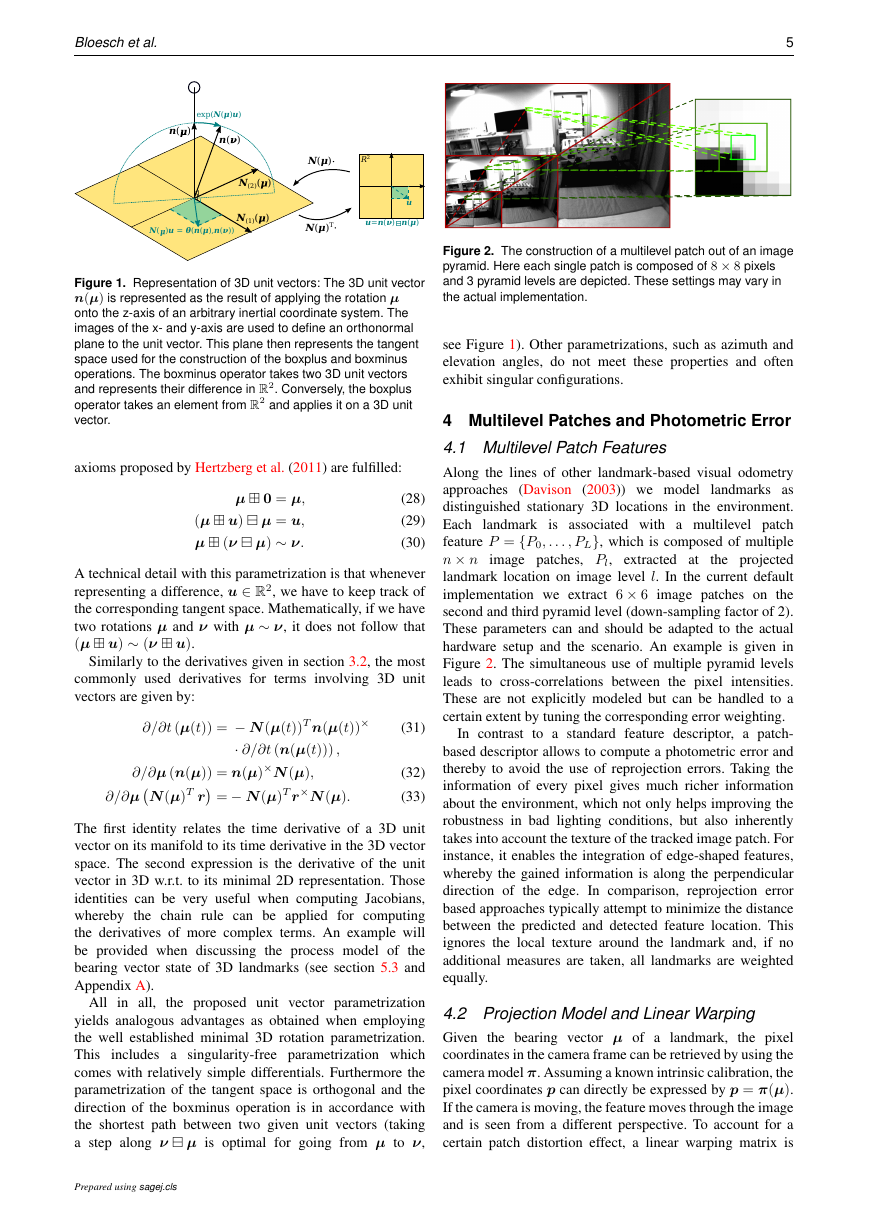
A visualization of the 2-sphere and the tangent space for a
specific µ is given in Figure 1.
The concept is slightly more complicated than in the case
of 3D rotations since we truly over-parameterize a 3D unit
vector (no constraint is imposed on the underlying rotation).
To overcome this, we use a different notion of equivalence
where we define that two unit vector parametrizations µ and
ν are equivalent (µ ∼ ν) iff n(µ) = n(ν). With this, the
�
Bloesch et al.
5
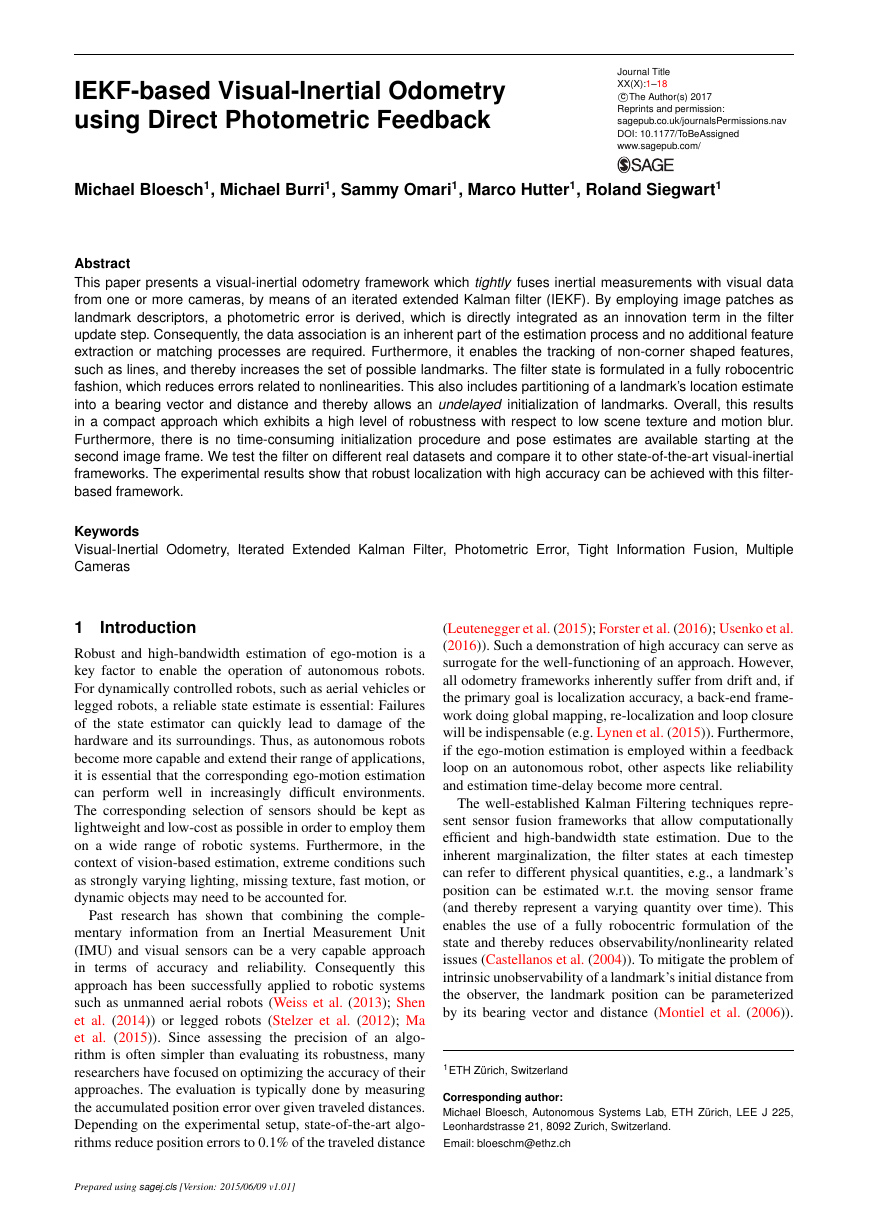
Figure 1. Representation of 3D unit vectors: The 3D unit vector
n(µ) is represented as the result of applying the rotation µ
onto the z-axis of an arbitrary inertial coordinate system. The
images of the x- and y-axis are used to define an orthonormal
plane to the unit vector. This plane then represents the tangent
space used for the construction of the boxplus and boxminus
operations. The boxminus operator takes two 3D unit vectors
and represents their difference in R2. Conversely, the boxplus
operator takes an element from R2 and applies it on a 3D unit
vector.
axioms proposed by Hertzberg et al. (2011) are fulfilled:
µ 0 = µ,
(µ u) µ = u,
µ (ν µ) ∼ ν.
(28)
(29)
(30)
A technical detail with this parametrization is that whenever
representing a difference, u ∈ R2, we have to keep track of
the corresponding tangent space. Mathematically, if we have
two rotations µ and ν with µ ∼ ν, it does not follow that
(µ u) ∼ (ν u).
Similarly to the derivatives given in section 3.2, the most
commonly used derivatives for terms involving 3D unit
vectors are given by:
∂/∂t (µ(t)) = − N (µ(t))T n(µ(t))×
∂/∂µ (n(µ)) = n(µ)×N (µ),
∂/∂µN (µ)T r = − N (µ)T r×N (µ).
· ∂/∂t (n(µ(t))) ,
(31)
(32)
(33)
The first identity relates the time derivative of a 3D unit
vector on its manifold to its time derivative in the 3D vector
space. The second expression is the derivative of the unit
vector in 3D w.r.t. to its minimal 2D representation. Those
identities can be very useful when computing Jacobians,
whereby the chain rule can be applied for computing
the derivatives of more complex terms. An example will
be provided when discussing the process model of the
bearing vector state of 3D landmarks (see section 5.3 and
Appendix A).
in all,
the proposed unit vector parametrization
yields analogous advantages as obtained when employing
the well established minimal 3D rotation parametrization.
This includes a singularity-free parametrization which
comes with relatively simple differentials. Furthermore the
parametrization of the tangent space is orthogonal and the
direction of the boxminus operation is in accordance with
the shortest path between two given unit vectors (taking
a step along ν µ is optimal for going from µ to ν,
All
Prepared using sagej.cls
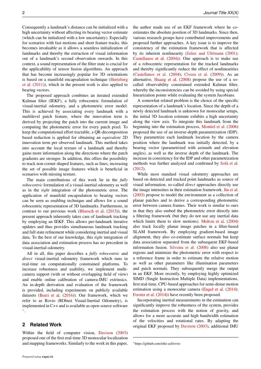
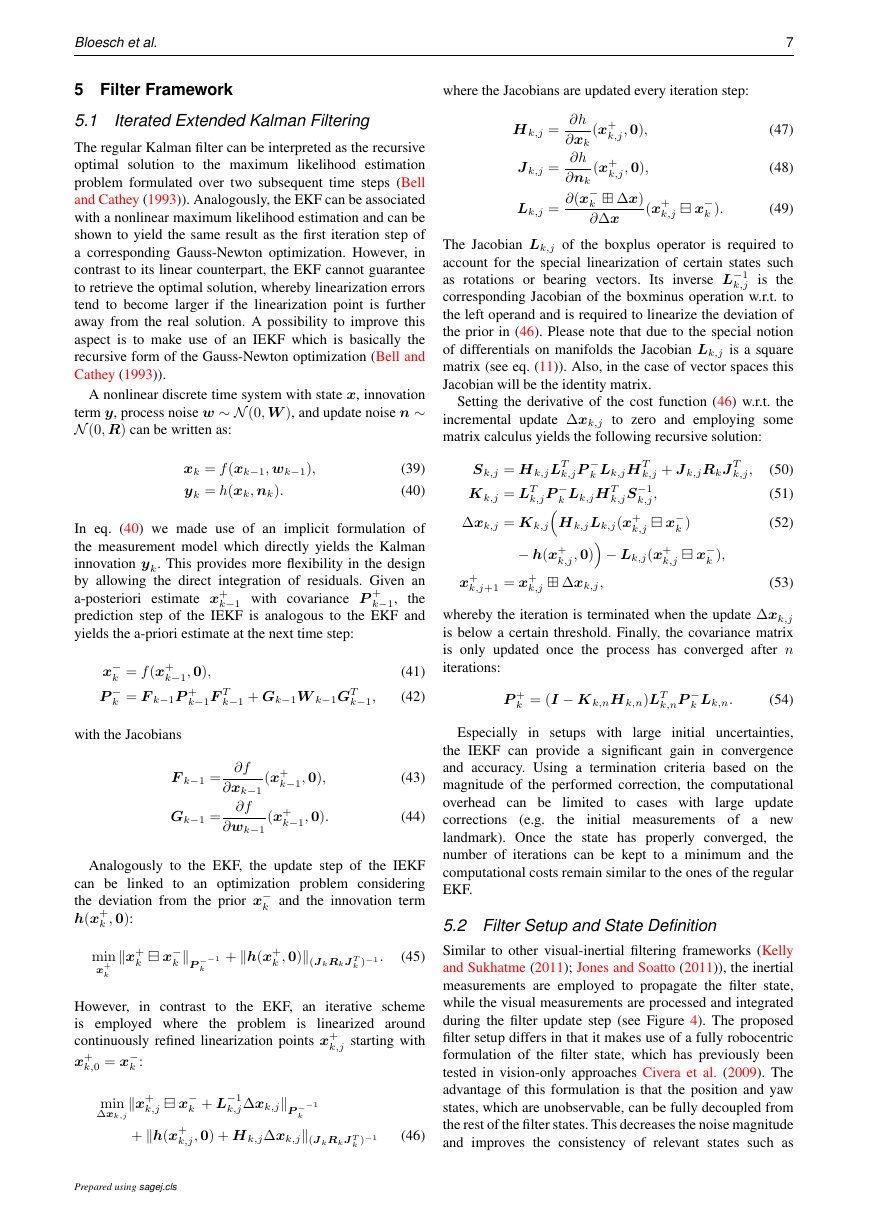
Figure 2. The construction of a multilevel patch out of an image
pyramid. Here each single patch is composed of 8 × 8 pixels
and 3 pyramid levels are depicted. These settings may vary in
the actual implementation.
see Figure 1). Other parametrizations, such as azimuth and
elevation angles, do not meet these properties and often
exhibit singular configurations.
4 Multilevel Patches and Photometric Error
4.1 Multilevel Patch Features
Along the lines of other landmark-based visual odometry
approaches (Davison (2003)) we model
landmarks as
distinguished stationary 3D locations in the environment.
Each landmark is associated with a multilevel patch
feature P = {P0, . . . , PL}, which is composed of multiple
n × n image patches, Pl, extracted at
the projected
landmark location on image level l. In the current default
implementation we extract 6 × 6 image patches on the
second and third pyramid level (down-sampling factor of 2).
These parameters can and should be adapted to the actual
hardware setup and the scenario. An example is given in
Figure 2. The simultaneous use of multiple pyramid levels
leads to cross-correlations between the pixel
intensities.
These are not explicitly modeled but can be handled to a
certain extent by tuning the corresponding error weighting.
to a standard feature descriptor, a patch-
based descriptor allows to compute a photometric error and
thereby to avoid the use of reprojection errors. Taking the
information of every pixel gives much richer information
about the environment, which not only helps improving the
robustness in bad lighting conditions, but also inherently
takes into account the texture of the tracked image patch. For
instance, it enables the integration of edge-shaped features,
whereby the gained information is along the perpendicular
direction of the edge. In comparison, reprojection error
based approaches typically attempt to minimize the distance
between the predicted and detected feature location. This
ignores the local texture around the landmark and, if no
additional measures are taken, all landmarks are weighted
equally.
In contrast
4.2 Projection Model and Linear Warping
Given the bearing vector µ of a landmark,
the pixel
coordinates in the camera frame can be retrieved by using the
camera model π. Assuming a known intrinsic calibration, the
pixel coordinates p can directly be expressed by p = π(µ).
If the camera is moving, the feature moves through the image
and is seen from a different perspective. To account for a
certain patch distortion effect, a linear warping matrix is
n()N(1)()N(2)()n()N(�)u = θ(n(μ),n(ν))exp(N(μ)u)N(μ)TN(μ)u=n(ν)�n(μ)R2u�
6
Journal Title XX(X)
tracked with each feature. This is done by concatenating
all Jacobians when transforming a landmark location. For
instance, if we detect a feature in some frame at pixel p1,
transform the corresponding bearing vector µ1 = π−1(p1)
with a process model µ2 = f (µ1), and then re-project the
bearing vector in a subsequent frame p2 = π(µ2), we obtain
the following linear warping matrix:
D =
∂π(µ2)
∂f (µ1)
∂π−1(p1)
∂µ2
∂µ1
∂p1
∈ R2×2.
(34)
In essence, this maps the two patch axes from the point of
patch extraction (which where aligned with the image axes)
to the two distorted patch axes in the projection image. This
approach tracks the distortion locally around the patch and
ignores any larger scale information like the geometric shape
of a patch. To avoid large distortions and the accumulation of
errors, the patches are re-extracted regularly and the warping
matrix is reset to identity.
4.3 Photometric Error and Patch Alignment
The photometric error between a given multilevel patch
feature and a specific image is computed by extracting
a warped patch at the estimated location and evaluating
the pixel-wise intensity error. For a given multilevel patch
feature (with coordinates p and multilevel patch P =
{P0, . . . , PL}) at a specific image level l and patch pixel pj,
the photometric error can be formalized as follows:
el,j(p, P, I, D) = Pl(pj) − a Il(p sl + Dpj) − b,
(35)
is the image at the pyramid level l and sl =
where Il
0.5l is a scaling factor to account for the down-sampling.
The linear warping matrix D is used to map patch pixel
coordinates to image coordinates. Furthermore, inter-frame
illumination changes are taken into account by employing
an affine intensity model composed of the scalars a and b
(both get marginalized out). Figure 3 depicts the photometric
error between a patch and its measurement in an image at a
predicted location p.
If we minimize the squared error terms for a multilevel
patch, we obtain a patch alignment algorithm which is
very similar to the well-known Kanade-Lucas-Tomasi (KLT)
feature tracker (Lucas and Kanade (1981); Shi and Tomasi
(1994)). A slight difference is given by the fact
that
we optimize over multiple image levels at once. The
minimization can be solved by a Gauss-Newton method
which iteratively linearizes the optimization problem around
an estimated patch location ˆp:
b(ˆp + δp, P, I, D) = A(ˆp, I, D)δp + b(ˆp, P, I, D),
(36)
where b(ˆp, P, I, D) represents the stacked error terms from
eq. (35) and A(ˆp, I, D) the corresponding Jacobian. The
corresponding normal equations are then given by:
A(ˆp, I, D)T A(ˆp, I, D)δp = −A(ˆp, I, D)T b(ˆp, P, I, D),
(37)
which can be solved for the correction δp. This is analogous
to one iteration step of the KLT feature tracker (but is not
used as such in Rovio). In section 5.4 we will demonstrate
Prepared using sagej.cls
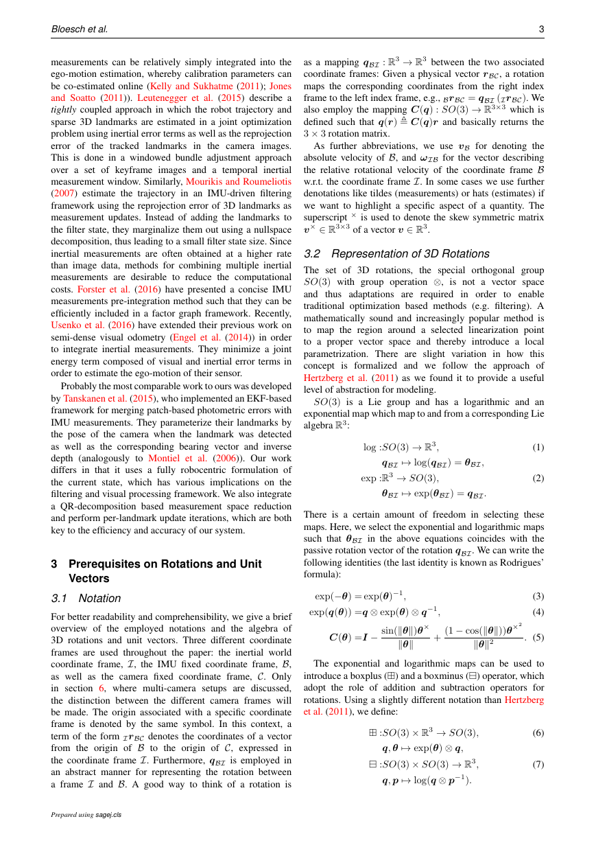
Figure 3. Illustration of the (signed) photometric error between
a previously extracted patch (green) and its projection into an
image (measured, red) at a predicted location p. The bottom left
grey tone of the difference patch represents 0. Only a single
image level is depicted. This photometric error is directly used
as the innovation term in an IEKF.
how eq. (36) is leveraged into the innovation term of the
employed IEKF.
Note that due to the scaling factor sl in eq. (35), error
terms for higher image levels will have a weaker corrective
influence on the filter state or the patch alignment. On the
other hand, they exhibit increased robustness w.r.t. image
blur or bad initial alignment and thus strongly increase the
robustness of the overall alignment method.
4.4 Detection and Scoring
The detection of new landmarks is based on the FAST corner
detector (Rosten and Drummond (2006)) which provides a
large amount of candidate feature locations. After removing
candidates which are close to currently tracked features,
we compute a patch gradient based score for selecting
new features which are added to the state. This basically
represents an adaptation of the Shi-Tomasi score (Shi and
Tomasi (1994)) by considering the combined Hessian on
multiple image levels, instead of only a single level. The
combined Hessian can be directly retrieved from the normal
equations (37):
H = A(ˆp, I, D)T A(ˆp, I, D),
(38)
where the minimal eigenvalue of H corresponds to the
adapted Shi-Tomasi score.
The advantage is that a high score is correlated with the
alignment accuracy of the corresponding multilevel patch
feature. Instead of returning the minimal eigenvalue, the
method can return other eigenvalue based scores like the
1- or 2-norm. This is useful in environments with scarce
corner data, whereby also edge-shaped features can be
considered. Finally, the detection process is also coupled
with a bucketing technique to achieve a good distribution of
the features within the camera frame.
�
Bloesch et al.
5 Filter Framework
5.1 Iterated Extended Kalman Filtering
The regular Kalman filter can be interpreted as the recursive
optimal solution to the maximum likelihood estimation
problem formulated over two subsequent time steps (Bell
and Cathey (1993)). Analogously, the EKF can be associated
with a nonlinear maximum likelihood estimation and can be
shown to yield the same result as the first iteration step of
a corresponding Gauss-Newton optimization. However, in
contrast to its linear counterpart, the EKF cannot guarantee
to retrieve the optimal solution, whereby linearization errors
tend to become larger if the linearization point is further
away from the real solution. A possibility to improve this
aspect is to make use of an IEKF which is basically the
recursive form of the Gauss-Newton optimization (Bell and
Cathey (1993)).
A nonlinear discrete time system with state x, innovation
term y, process noise w ∼ N (0, W ), and update noise n ∼
N (0, R) can be written as:
xk = f (xk−1, wk−1),
yk = h(xk, nk).
(39)
(40)
In eq. (40) we made use of an implicit formulation of
the measurement model which directly yields the Kalman
innovation yk. This provides more flexibility in the design
by allowing the direct integration of residuals. Given an
a-posteriori estimate x+
the
prediction step of the IEKF is analogous to the EKF and
yields the a-priori estimate at the next time step:
k−1 with covariance P +
k−1,
x−
k = f (x+
P −
k = F k−1P +
k−1, 0),
k−1F T
k−1 + Gk−1W k−1GT
k−1,
with the Jacobians
F k−1 =
Gk−1 =
∂f
∂xk−1
∂f
∂wk−1
(x+
k−1, 0),
(x+
k−1, 0).
(41)
(42)
(43)
(44)
Analogously to the EKF, the update step of the IEKF
can be linked to an optimization problem considering
the deviation from the prior x−
k and the innovation term
h(x+
k , 0):
min
x+
k x+
k
x−
k P
−−1
k
+ h(x+
k , 0)(J kRkJ T
k )−1 .
(45)
in contrast
However,
to the EKF, an iterative scheme
is employed where the problem is linearized around
continuously refined linearization points x+
k,j starting with
k,0 = x−
x+
k :
∆xk,jx+
min
k,j
x−
k,j∆xk,jP
k + L−1
k,j, 0) + H k,j∆xk,j(J kRkJ T
−−1
k
+ h(x+
k )−1
(46)
Prepared using sagej.cls
where the Jacobians are updated every iteration step:
H k,j =
J k,j =
Lk,j =
∂h
∂xk
∂h
∂nk
∂(x−
(x+
k,j, 0),
(x+
k,j, 0),
∆x)
k
∂∆x
(x+
k,j
x−
k ).
7
(47)
(48)
(49)
The Jacobian Lk,j of the boxplus operator is required to
account for the special linearization of certain states such
as rotations or bearing vectors. Its inverse L−1
is the
corresponding Jacobian of the boxminus operation w.r.t. to
the left operand and is required to linearize the deviation of
the prior in (46). Please note that due to the special notion
of differentials on manifolds the Jacobian Lk,j is a square
matrix (see eq. (11)). Also, in the case of vector spaces this
Jacobian will be the identity matrix.
k,j
Setting the derivative of the cost function (46) w.r.t. the
incremental update ∆xk,j to zero and employing some
matrix calculus yields the following recursive solution:
Sk,j = H k,jLT
k,jP −
Kk,j = LT
− h(x+
∆xk,j = Kk,j
k,jP −
k,j + J k,jRkJ T
k Lk,jH T
k,jS−1
k Lk,jH T
k,j,
H k,jLk,j(x+
k,j
x−
k )
x−
k ),
− Lk,j(x+
k,j
k,j,
x+
k,j+1 = x+
k,j
k,j, 0)
∆xk,j,
(50)
(51)
(52)
(53)
whereby the iteration is terminated when the update ∆xk,j
is below a certain threshold. Finally, the covariance matrix
is only updated once the process has converged after n
iterations:
k = (I − Kk,nH k,n)LT
P +
k,nP −
k Lk,n.
(54)
Especially in setups with large initial uncertainties,
the IEKF can provide a significant gain in convergence
and accuracy. Using a termination criteria based on the
magnitude of the performed correction, the computational
overhead can be limited to cases with large update
the initial measurements of a new
corrections
landmark). Once the state has properly converged,
the
number of iterations can be kept to a minimum and the
computational costs remain similar to the ones of the regular
EKF.
(e.g.
5.2 Filter Setup and State Definition
Similar to other visual-inertial filtering frameworks (Kelly
and Sukhatme (2011); Jones and Soatto (2011)), the inertial
measurements are employed to propagate the filter state,
while the visual measurements are processed and integrated
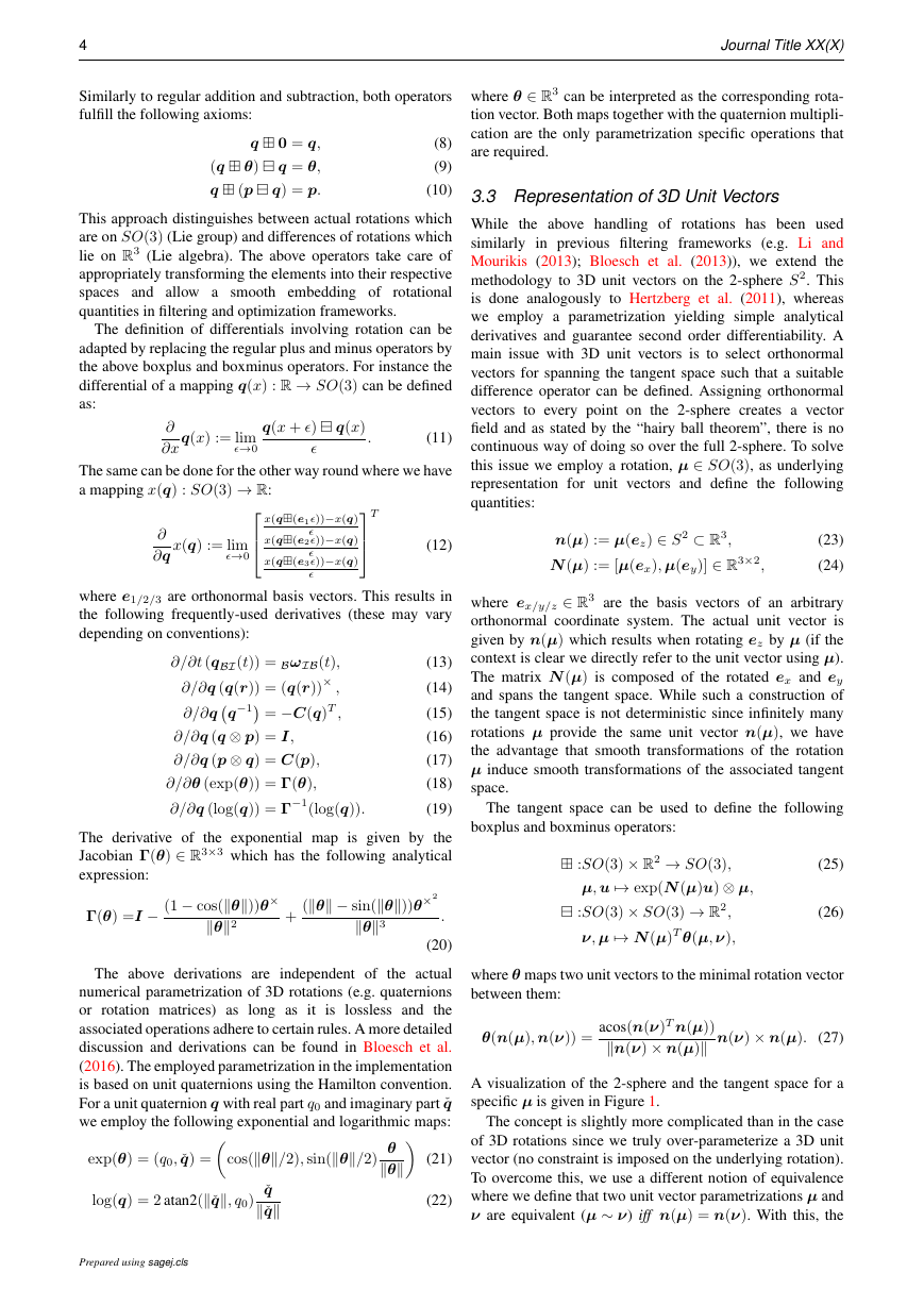
during the filter update step (see Figure 4). The proposed
filter setup differs in that it makes use of a fully robocentric
formulation of the filter state, which has previously been
tested in vision-only approaches Civera et al. (2009). The
advantage of this formulation is that the position and yaw
states, which are unobservable, can be fully decoupled from
the rest of the filter states. This decreases the noise magnitude
and improves the consistency of relevant states such as
�




 2023年江西萍乡中考道德与法治真题及答案.doc
 2012年重庆南川中考生物真题及答案.doc
 2013年江西师范大学地理学综合及文艺理论基础考研真题.doc
 2020年四川甘孜小升初语文真题及答案I卷.doc
 2020年注册岩土工程师专业基础考试真题及答案.doc
 2023-2024学年福建省厦门市九年级上学期数学月考试题及答案.doc
 2021-2022学年辽宁省沈阳市大东区九年级上学期语文期末试题及答案.doc
 2022-2023学年北京东城区初三第一学期物理期末试卷及答案.doc
 2018上半年江西教师资格初中地理学科知识与教学能力真题及答案.doc
 2012年河北国家公务员申论考试真题及答案-省级.doc
 2020-2021学年江苏省扬州市江都区邵樊片九年级上学期数学第一次质量检测试题及答案.doc
 2022下半年黑龙江教师资格证中学综合素质真题及答案.doc