Resilient Distributed Datasets: A Fault-Tolerant Abstraction for
In-Memory Cluster Computing
Matei Zaharia, Mosharaf Chowdhury, Tathagata Das, Ankur Dave, Justin Ma,
Murphy McCauley, Michael J. Franklin, Scott Shenker, Ion Stoica
University of California, Berkeley
Abstract
We present Resilient Distributed Datasets (RDDs), a dis-
tributed memory abstraction that lets programmers per-
form in-memory computations on large clusters in a
fault-tolerant manner. RDDs are motivated by two types
of applications that current computing frameworks han-
dle inefficiently: iterative algorithms and interactive data
mining tools. In both cases, keeping data in memory
can improve performance by an order of magnitude.
To achieve fault tolerance efficiently, RDDs provide a
restricted form of shared memory, based on coarse-
grained transformations rather than fine-grained updates
to shared state. However, we show that RDDs are expres-
sive enough to capture a wide class of computations, in-
cluding recent specialized programming models for iter-
ative jobs, such as Pregel, and new applications that these
models do not capture. We have implemented RDDs in a
system called Spark, which we evaluate through a variety
of user applications and benchmarks.
1
Cluster computing frameworks like MapReduce [10] and
Dryad [19] have been widely adopted for large-scale data
analytics. These systems let users write parallel compu-
tations using a set of high-level operators, without having
to worry about work distribution and fault tolerance.
Introduction
Although current frameworks provide numerous ab-
stractions for accessing a cluster’s computational re-
sources, they lack abstractions for leveraging distributed
memory. This makes them inefficient for an important
class of emerging applications: those that reuse interme-
diate results across multiple computations. Data reuse is
common in many iterative machine learning and graph
algorithms, including PageRank, K-means clustering,
and logistic regression. Another compelling use case is
interactive data mining, where a user runs multiple ad-
hoc queries on the same subset of the data. Unfortu-
nately, in most current frameworks, the only way to reuse
data between computations (e.g., between two MapRe-
duce jobs) is to write it to an external stable storage sys-
tem, e.g., a distributed file system. This incurs substantial
overheads due to data replication, disk I/O, and serializa-
tion, which can dominate application execution times.
Recognizing this problem, researchers have developed
specialized frameworks for some applications that re-
quire data reuse. For example, Pregel [22] is a system for
iterative graph computations that keeps intermediate data
in memory, while HaLoop [7] offers an iterative MapRe-
duce interface. However, these frameworks only support
specific computation patterns (e.g., looping a series of
MapReduce steps), and perform data sharing implicitly
for these patterns. They do not provide abstractions for
more general reuse, e.g., to let a user load several datasets
into memory and run ad-hoc queries across them.
In this paper, we propose a new abstraction called re-
silient distributed datasets (RDDs) that enables efficient
data reuse in a broad range of applications. RDDs are
fault-tolerant, parallel data structures that let users ex-
plicitly persist intermediate results in memory, control
their partitioning to optimize data placement, and ma-
nipulate them using a rich set of operators.
The main challenge in designing RDDs is defining a
programming interface that can provide fault tolerance
efficiently. Existing abstractions for in-memory storage
on clusters, such as distributed shared memory [24], key-
value stores [25], databases, and Piccolo [27], offer an
interface based on fine-grained updates to mutable state
(e.g., cells in a table). With this interface, the only ways
to provide fault tolerance are to replicate the data across
machines or to log updates across machines. Both ap-
proaches are expensive for data-intensive workloads, as
they require copying large amounts of data over the clus-
ter network, whose bandwidth is far lower than that of
RAM, and they incur substantial storage overhead.
In contrast to these systems, RDDs provide an inter-
face based on coarse-grained transformations (e.g., map,
filter and join) that apply the same operation to many
data items. This allows them to efficiently provide fault
tolerance by logging the transformations used to build a
dataset (its lineage) rather than the actual data.1 If a parti-
tion of an RDD is lost, the RDD has enough information
about how it was derived from other RDDs to recompute
1Checkpointing the data in some RDDs may be useful when a lin-
eage chain grows large, however, and we discuss how to do it in §5.4.
�
just that partition. Thus, lost data can be recovered, often
quite quickly, without requiring costly replication.
Although an interface based on coarse-grained trans-
formations may at first seem limited, RDDs are a good
fit for many parallel applications, because these appli-
cations naturally apply the same operation to multiple
data items. Indeed, we show that RDDs can efficiently
express many cluster programming models that have so
far been proposed as separate systems, including MapRe-
duce, DryadLINQ, SQL, Pregel and HaLoop, as well as
new applications that these systems do not capture, like
interactive data mining. The ability of RDDs to accom-
modate computing needs that were previously met only
by introducing new frameworks is, we believe, the most
credible evidence of the power of the RDD abstraction.
We have implemented RDDs in a system called Spark,
which is being used for research and production applica-
tions at UC Berkeley and several companies. Spark pro-
vides a convenient language-integrated programming in-
terface similar to DryadLINQ [31] in the Scala program-
ming language [2]. In addition, Spark can be used inter-
actively to query big datasets from the Scala interpreter.
We believe that Spark is the first system that allows a
general-purpose programming language to be used at in-
teractive speeds for in-memory data mining on clusters.
We evaluate RDDs and Spark through both mi-
crobenchmarks and measurements of user applications.
We show that Spark is up to 20× faster than Hadoop for
iterative applications, speeds up a real-world data analyt-
ics report by 40×, and can be used interactively to scan a
1 TB dataset with 5–7s latency. More fundamentally, to
illustrate the generality of RDDs, we have implemented
the Pregel and HaLoop programming models on top of
Spark, including the placement optimizations they em-
ploy, as relatively small libraries (200 lines of code each).
This paper begins with an overview of RDDs (§2) and
Spark (§3). We then discuss the internal representation
of RDDs (§4), our implementation (§5), and experimen-
tal results (§6). Finally, we discuss how RDDs capture
several existing cluster programming models (§7), sur-
vey related work (§8), and conclude.
2 Resilient Distributed Datasets (RDDs)
This section provides an overview of RDDs. We first de-
fine RDDs (§2.1) and introduce their programming inter-
face in Spark (§2.2). We then compare RDDs with finer-
grained shared memory abstractions (§2.3). Finally, we
discuss limitations of the RDD model (§2.4).
2.1 RDD Abstraction
Formally, an RDD is a read-only, partitioned collection
of records. RDDs can only be created through determin-
istic operations on either (1) data in stable storage or (2)
other RDDs. We call these operations transformations to
differentiate them from other operations on RDDs. Ex-
amples of transformations include map, filter, and join.2
RDDs do not need to be materialized at all times. In-
stead, an RDD has enough information about how it was
derived from other datasets (its lineage) to compute its
partitions from data in stable storage. This is a power-
ful property: in essence, a program cannot reference an
RDD that it cannot reconstruct after a failure.
Finally, users can control two other aspects of RDDs:
persistence and partitioning. Users can indicate which
RDDs they will reuse and choose a storage strategy for
them (e.g., in-memory storage). They can also ask that
an RDD’s elements be partitioned across machines based
on a key in each record. This is useful for placement op-
timizations, such as ensuring that two datasets that will
be joined together are hash-partitioned in the same way.
2.2 Spark Programming Interface
Spark exposes RDDs through a language-integrated API
similar to DryadLINQ [31] and FlumeJava [8], where
each dataset is represented as an object and transforma-
tions are invoked using methods on these objects.
Programmers start by defining one or more RDDs
through transformations on data in stable storage
(e.g., map and filter). They can then use these RDDs in
actions, which are operations that return a value to the
application or export data to a storage system. Examples
of actions include count (which returns the number of
elements in the dataset), collect (which returns the ele-
ments themselves), and save (which outputs the dataset
to a storage system). Like DryadLINQ, Spark computes
RDDs lazily the first time they are used in an action, so
that it can pipeline transformations.
In addition, programmers can call a persist method to
indicate which RDDs they want to reuse in future oper-
ations. Spark keeps persistent RDDs in memory by de-
fault, but it can spill them to disk if there is not enough
RAM. Users can also request other persistence strategies,
such as storing the RDD only on disk or replicating it
across machines, through flags to persist. Finally, users
can set a persistence priority on each RDD to specify
which in-memory data should spill to disk first.
2.2.1 Example: Console Log Mining
Suppose that a web service is experiencing errors and an
operator wants to search terabytes of logs in the Hadoop
filesystem (HDFS) to find the cause. Using Spark, the op-
erator can load just the error messages from the logs into
RAM across a set of nodes and query them interactively.
She would first type the following Scala code:
2Although individual RDDs are immutable, it is possible to imple-
ment mutable state by having multiple RDDs to represent multiple ver-
sions of a dataset. We made RDDs immutable to make it easier to de-
scribe lineage graphs, but it would have been equivalent to have our
abstraction be versioned datasets and track versions in lineage graphs.
�
Figure 1: Lineage graph for the third query in our example.
Boxes represent RDDs and arrows represent transformations.
lines = spark.textFile("hdfs://...")
errors = lines.filter(_.startsWith("ERROR"))
errors.persist()
Line 1 defines an RDD backed by an HDFS file (as a
collection of lines of text), while line 2 derives a filtered
RDD from it. Line 3 then asks for errors to persist in
memory so that it can be shared across queries. Note that
the argument to filter is Scala syntax for a closure.
At this point, no work has been performed on the clus-
ter. However, the user can now use the RDD in actions,
e.g., to count the number of messages:
errors.count()
The user can also perform further transformations on
the RDD and use their results, as in the following lines:
// Count errors mentioning MySQL:
errors.filter(_.contains("MySQL")).count()
// Return the time fields of errors mentioning
// HDFS as an array (assuming time is field
// number 3 in a tab-separated format):
errors.filter(_.contains("HDFS"))
.map(_.split(’\t’)(3))
.collect()
After the first action involving errors runs, Spark will
store the partitions of errors in memory, greatly speed-
ing up subsequent computations on it. Note that the base
RDD, lines, is not loaded into RAM. This is desirable
because the error messages might only be a small frac-
tion of the data (small enough to fit into memory).
Finally, to illustrate how our model achieves fault tol-
erance, we show the lineage graph for the RDDs in our
third query in Figure 1. In this query, we started with
errors, the result of a filter on lines, and applied a fur-
ther filter and map before running a collect. The Spark
scheduler will pipeline the latter two transformations and
send a set of tasks to compute them to the nodes holding
the cached partitions of errors. In addition, if a partition
of errors is lost, Spark rebuilds it by applying a filter on
only the corresponding partition of lines.
Table 1: Comparison of RDDs with distributed shared memory.
2.3 Advantages of the RDD Model
To understand the benefits of RDDs as a distributed
memory abstraction, we compare them against dis-
tributed shared memory (DSM) in Table 1. In DSM sys-
tems, applications read and write to arbitrary locations in
a global address space. Note that under this definition, we
include not only traditional shared memory systems [24],
but also other systems where applications make fine-
grained writes to shared state, including Piccolo [27],
which provides a shared DHT, and distributed databases.
DSM is a very general abstraction, but this generality
makes it harder to implement in an efficient and fault-
tolerant manner on commodity clusters.
The main difference between RDDs and DSM is that
RDDs can only be created (“written”) through coarse-
grained transformations, while DSM allows reads and
writes to each memory location.3 This restricts RDDs
to applications that perform bulk writes, but allows for
more efficient fault tolerance. In particular, RDDs do not
need to incur the overhead of checkpointing, as they can
be recovered using lineage.4 Furthermore, only the lost
partitions of an RDD need to be recomputed upon fail-
ure, and they can be recomputed in parallel on different
nodes, without having to roll back the whole program.
A second benefit of RDDs is that their immutable na-
ture lets a system mitigate slow nodes (stragglers) by run-
ning backup copies of slow tasks as in MapReduce [10].
Backup tasks would be hard to implement with DSM, as
the two copies of a task would access the same memory
locations and interfere with each other’s updates.
Finally, RDDs provide two other benefits over DSM.
First, in bulk operations on RDDs, a runtime can sched-
3Note that reads on RDDs can still be fine-grained. For example, an
application can treat an RDD as a large read-only lookup table.
4In some applications, it can still help to checkpoint RDDs with
long lineage chains, as we discuss in Section 5.4. However, this can be
done in the background because RDDs are immutable, and there is no
need to take a snapshot of the whole application as in DSM.
lines errors filter(_.startsWith(“ERROR”)) HDFS errors time fields filter(_.contains(“HDFS”))) map(_.split(‘\t’)(3)) Aspect RDDs Distr. Shared Mem. Reads Coarse- or fine-grained Fine-grained Writes Coarse-grained Fine-grained Consistency Trivial (immutable) Up to app / runtime Fault recovery Fine-grained and low-overhead using lineage Requires checkpoints and program rollback Straggler mitigation Possible using backup tasks Difficult Work placement Automatic based on data locality Up to app (runtimes aim for transparency) Behavior if not enough RAM Similar to existing data flow systems Poor performance (swapping?) �
tions like map by passing closures (function literals).
Scala represents each closure as a Java object, and
these objects can be serialized and loaded on another
node to pass the closure across the network. Scala also
saves any variables bound in the closure as fields in
the Java object. For example, one can write code like
var x = 5; rdd.map(_ + x) to add 5 to each element
of an RDD.5
RDDs
are
themselves
statically typed objects
parametrized by an element
type. For example,
RDD[Int] is an RDD of integers. However, most of our
examples omit types since Scala supports type inference.
Although our method of exposing RDDs in Scala is
conceptually simple, we had to work around issues with
Scala’s closure objects using reflection [33]. We also
needed more work to make Spark usable from the Scala
interpreter, as we shall discuss in Section 5.2. Nonethe-
less, we did not have to modify the Scala compiler.
3.1 RDD Operations in Spark
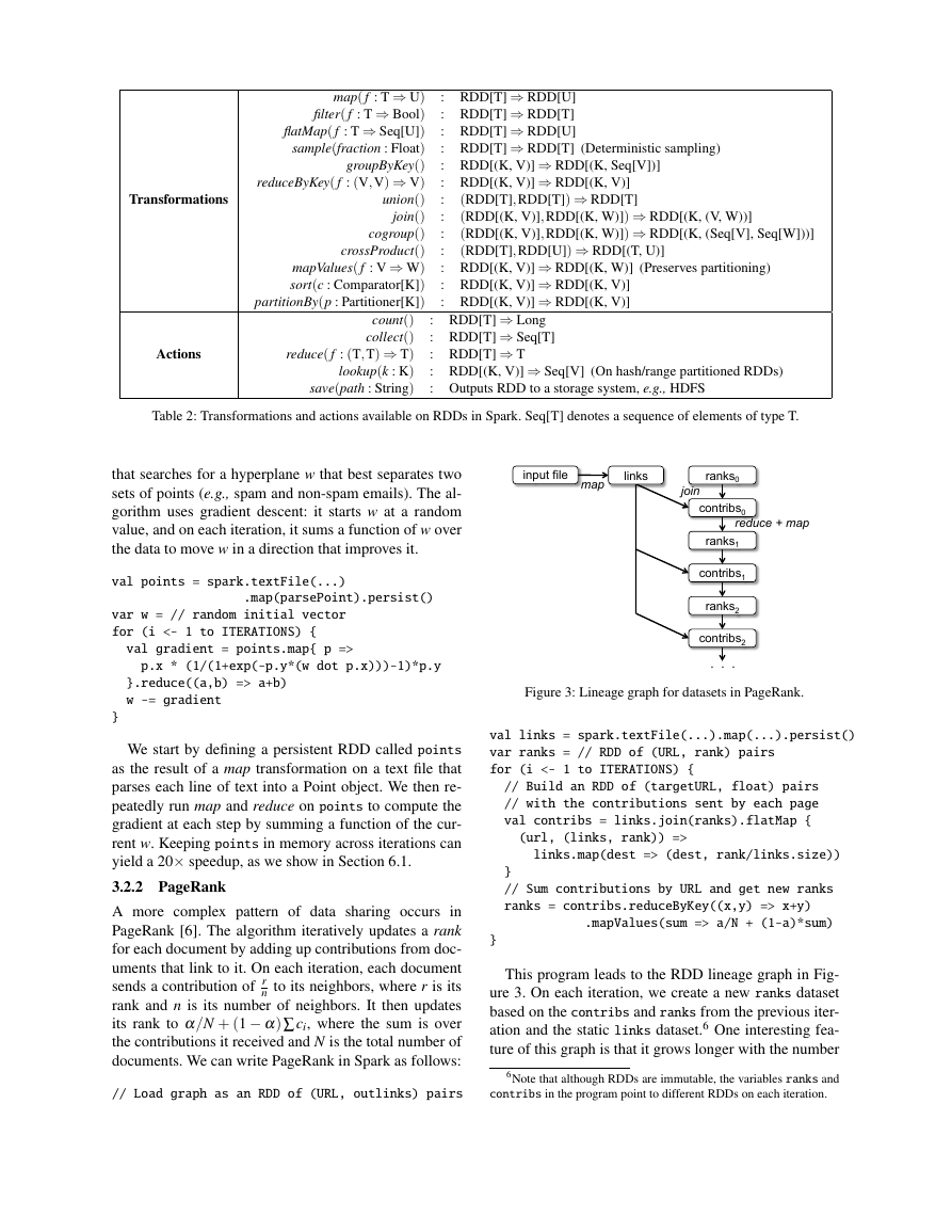
Table 2 lists the main RDD transformations and actions
available in Spark. We give the signature of each oper-
ation, showing type parameters in square brackets. Re-
call that transformations are lazy operations that define a
new RDD, while actions launch a computation to return
a value to the program or write data to external storage.
Note that some operations, such as join, are only avail-
able on RDDs of key-value pairs. Also, our function
names are chosen to match other APIs in Scala and other
functional languages; for example, map is a one-to-one
mapping, while flatMap maps each input value to one or
more outputs (similar to the map in MapReduce).
In addition to these operators, users can ask for an
RDD to persist. Furthermore, users can get an RDD’s
partition order, which is represented by a Partitioner
class, and partition another dataset according to it. Op-
erations such as groupByKey, reduceByKey and sort au-
tomatically result in a hash or range partitioned RDD.
3.2 Example Applications
We complement the data mining example in Section
2.2.1 with two iterative applications: logistic regression
and PageRank. The latter also showcases how control of
RDDs’ partitioning can improve performance.
3.2.1 Logistic Regression
Many machine learning algorithms are iterative in nature
because they run iterative optimization procedures, such
as gradient descent, to maximize a function. They can
thus run much faster by keeping their data in memory.
As an example, the following program implements lo-
gistic regression [14], a common classification algorithm
5We save each closure at the time it is created, so that the map in
this example will always add 5 even if x changes.
Figure 2: Spark runtime. The user’s driver program launches
multiple workers, which read data blocks from a distributed file
system and can persist computed RDD partitions in memory.
ule tasks based on data locality to improve performance.
Second, RDDs degrade gracefully when there is not
enough memory to store them, as long as they are only
being used in scan-based operations. Partitions that do
not fit in RAM can be stored on disk and will provide
similar performance to current data-parallel systems.
2.4 Applications Not Suitable for RDDs
As discussed in the Introduction, RDDs are best suited
for batch applications that apply the same operation to
all elements of a dataset. In these cases, RDDs can ef-
ficiently remember each transformation as one step in a
lineage graph and can recover lost partitions without hav-
ing to log large amounts of data. RDDs would be less
suitable for applications that make asynchronous fine-
grained updates to shared state, such as a storage sys-
tem for a web application or an incremental web crawler.
For these applications, it is more efficient to use systems
that perform traditional update logging and data check-
pointing, such as databases, RAMCloud [25], Percolator
[26] and Piccolo [27]. Our goal is to provide an efficient
programming model for batch analytics and leave these
asynchronous applications to specialized systems.
3 Spark Programming Interface
Spark provides the RDD abstraction through a language-
integrated API similar to DryadLINQ [31] in Scala [2],
a statically typed functional programming language for
the Java VM. We chose Scala due to its combination of
conciseness (which is convenient for interactive use) and
efficiency (due to static typing). However, nothing about
the RDD abstraction requires a functional language.
To use Spark, developers write a driver program that
connects to a cluster of workers, as shown in Figure 2.
The driver defines one or more RDDs and invokes ac-
tions on them. Spark code on the driver also tracks the
RDDs’ lineage. The workers are long-lived processes
that can store RDD partitions in RAM across operations.
As we showed in the log mining example in Sec-
tion 2.2.1, users provide arguments to RDD opera-
Worker tasks results RAM Input Data Worker RAM Input Data Worker RAM Input Data Driver �
map( f : T ⇒ U)
filter( f : T ⇒ Bool)
flatMap( f : T ⇒ Seq[U])
sample(fraction : Float)
groupByKey()
reduceByKey( f : (V,V) ⇒ V)
union()
join()
cogroup()
crossProduct()
mapValues( f : V ⇒ W)
sort(c : Comparator[K])
partitionBy(p : Partitioner[K])
count()
collect()
reduce( f : (T,T) ⇒ T)
lookup(k : K)
save(path : String)
: RDD[T] ⇒ RDD[U]
: RDD[T] ⇒ RDD[T]
: RDD[T] ⇒ RDD[U]
: RDD[T] ⇒ RDD[T] (Deterministic sampling)
: RDD[(K, V)] ⇒ RDD[(K, Seq[V])]
: RDD[(K, V)] ⇒ RDD[(K, V)]
(RDD[T],RDD[T]) ⇒ RDD[T]
:
(RDD[(K, V)],RDD[(K, W)]) ⇒ RDD[(K, (V, W))]
:
(RDD[(K, V)],RDD[(K, W)]) ⇒ RDD[(K, (Seq[V], Seq[W]))]
:
(RDD[T],RDD[U]) ⇒ RDD[(T, U)]
:
: RDD[(K, V)] ⇒ RDD[(K, W)] (Preserves partitioning)
: RDD[(K, V)] ⇒ RDD[(K, V)]
: RDD[(K, V)] ⇒ RDD[(K, V)]
: RDD[T] ⇒ Long
: RDD[T] ⇒ Seq[T]
: RDD[T] ⇒ T
: RDD[(K, V)] ⇒ Seq[V] (On hash/range partitioned RDDs)
: Outputs RDD to a storage system, e.g., HDFS
Transformations
Actions
Table 2: Transformations and actions available on RDDs in Spark. Seq[T] denotes a sequence of elements of type T.
that searches for a hyperplane w that best separates two
sets of points (e.g., spam and non-spam emails). The al-
gorithm uses gradient descent: it starts w at a random
value, and on each iteration, it sums a function of w over
the data to move w in a direction that improves it.
val points = spark.textFile(...)
.map(parsePoint).persist()
var w = // random initial vector
for (i <- 1 to ITERATIONS) {
val gradient = points.map{ p =>
p.x * (1/(1+exp(-p.y*(w dot p.x)))-1)*p.y
}.reduce((a,b) => a+b)
w -= gradient
}
We start by defining a persistent RDD called points
as the result of a map transformation on a text file that
parses each line of text into a Point object. We then re-
peatedly run map and reduce on points to compute the
gradient at each step by summing a function of the cur-
rent w. Keeping points in memory across iterations can
yield a 20× speedup, as we show in Section 6.1.
3.2.2 PageRank
A more complex pattern of data sharing occurs in
PageRank [6]. The algorithm iteratively updates a rank
for each document by adding up contributions from doc-
uments that link to it. On each iteration, each document
sends a contribution of r
n to its neighbors, where r is its
rank and n is its number of neighbors. It then updates
its rank to α/N + (1 − α)∑ci, where the sum is over
the contributions it received and N is the total number of
documents. We can write PageRank in Spark as follows:
// Load graph as an RDD of (URL, outlinks) pairs
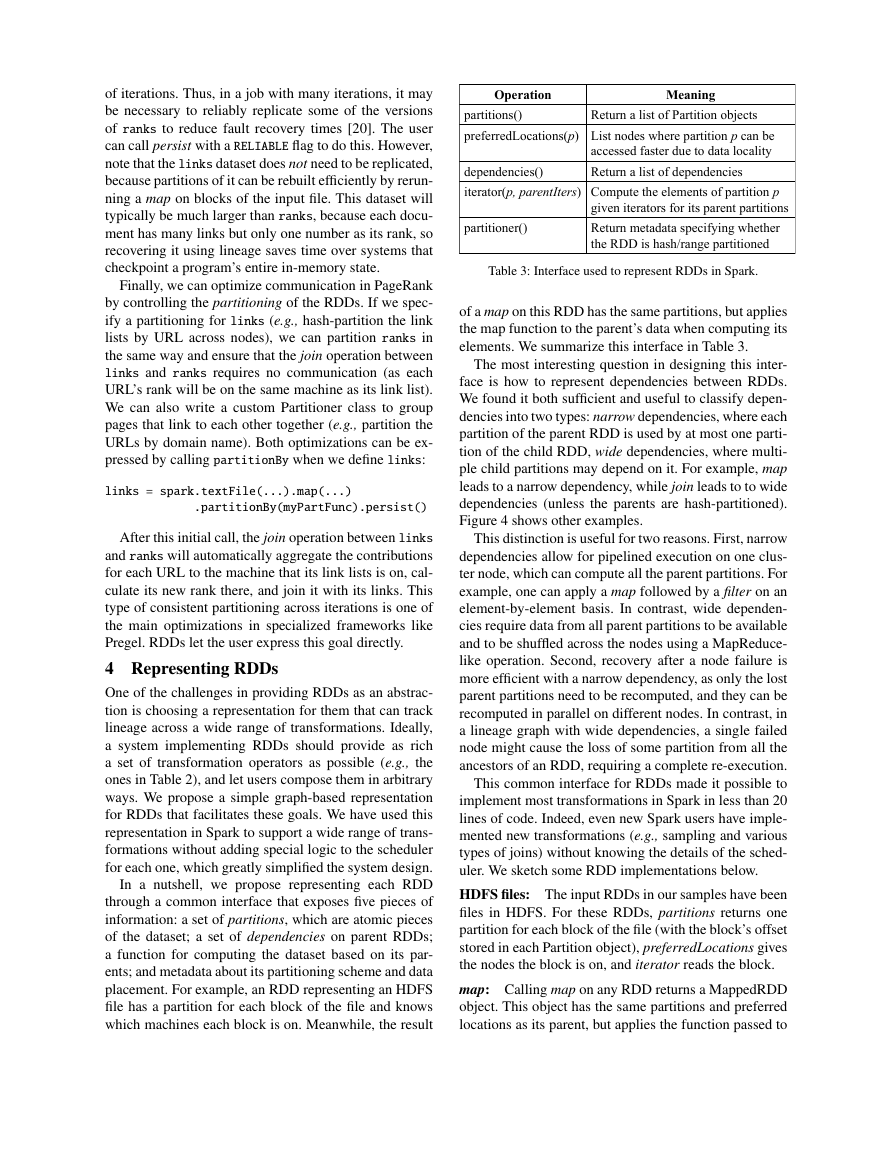
Figure 3: Lineage graph for datasets in PageRank.
val links = spark.textFile(...).map(...).persist()
var ranks = // RDD of (URL, rank) pairs
for (i <- 1 to ITERATIONS) {
// Build an RDD of (targetURL, float) pairs
// with the contributions sent by each page
val contribs = links.join(ranks).flatMap {
(url, (links, rank)) =>
links.map(dest => (dest, rank/links.size))
}
// Sum contributions by URL and get new ranks
ranks = contribs.reduceByKey((x,y) => x+y)
.mapValues(sum => a/N + (1-a)*sum)
}
This program leads to the RDD lineage graph in Fig-
ure 3. On each iteration, we create a new ranks dataset
based on the contribs and ranks from the previous iter-
ation and the static links dataset.6 One interesting fea-
ture of this graph is that it grows longer with the number
6Note that although RDDs are immutable, the variables ranks and
contribs in the program point to different RDDs on each iteration.
ranks0 input file map contribs0 ranks1 contribs1 ranks2 contribs2 links join reduce + map . . . �
of iterations. Thus, in a job with many iterations, it may
be necessary to reliably replicate some of the versions
of ranks to reduce fault recovery times [20]. The user
can call persist with a RELIABLE flag to do this. However,
note that the links dataset does not need to be replicated,
because partitions of it can be rebuilt efficiently by rerun-
ning a map on blocks of the input file. This dataset will
typically be much larger than ranks, because each docu-
ment has many links but only one number as its rank, so
recovering it using lineage saves time over systems that
checkpoint a program’s entire in-memory state.
Finally, we can optimize communication in PageRank
by controlling the partitioning of the RDDs. If we spec-
ify a partitioning for links (e.g., hash-partition the link
lists by URL across nodes), we can partition ranks in
the same way and ensure that the join operation between
links and ranks requires no communication (as each
URL’s rank will be on the same machine as its link list).
We can also write a custom Partitioner class to group
pages that link to each other together (e.g., partition the
URLs by domain name). Both optimizations can be ex-
pressed by calling partitionBy when we define links:
links = spark.textFile(...).map(...)
.partitionBy(myPartFunc).persist()
After this initial call, the join operation between links
and ranks will automatically aggregate the contributions
for each URL to the machine that its link lists is on, cal-
culate its new rank there, and join it with its links. This
type of consistent partitioning across iterations is one of
the main optimizations in specialized frameworks like
Pregel. RDDs let the user express this goal directly.
4 Representing RDDs
One of the challenges in providing RDDs as an abstrac-
tion is choosing a representation for them that can track
lineage across a wide range of transformations. Ideally,
a system implementing RDDs should provide as rich
a set of transformation operators as possible (e.g., the
ones in Table 2), and let users compose them in arbitrary
ways. We propose a simple graph-based representation
for RDDs that facilitates these goals. We have used this
representation in Spark to support a wide range of trans-
formations without adding special logic to the scheduler
for each one, which greatly simplified the system design.
In a nutshell, we propose representing each RDD
through a common interface that exposes five pieces of
information: a set of partitions, which are atomic pieces
of the dataset; a set of dependencies on parent RDDs;
a function for computing the dataset based on its par-
ents; and metadata about its partitioning scheme and data
placement. For example, an RDD representing an HDFS
file has a partition for each block of the file and knows
which machines each block is on. Meanwhile, the result
Table 3: Interface used to represent RDDs in Spark.
of a map on this RDD has the same partitions, but applies
the map function to the parent’s data when computing its
elements. We summarize this interface in Table 3.
The most interesting question in designing this inter-
face is how to represent dependencies between RDDs.
We found it both sufficient and useful to classify depen-
dencies into two types: narrow dependencies, where each
partition of the parent RDD is used by at most one parti-
tion of the child RDD, wide dependencies, where multi-
ple child partitions may depend on it. For example, map
leads to a narrow dependency, while join leads to to wide
dependencies (unless the parents are hash-partitioned).
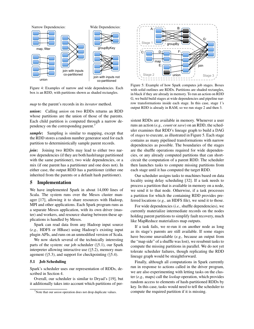
Figure 4 shows other examples.
This distinction is useful for two reasons. First, narrow
dependencies allow for pipelined execution on one clus-
ter node, which can compute all the parent partitions. For
example, one can apply a map followed by a filter on an
element-by-element basis. In contrast, wide dependen-
cies require data from all parent partitions to be available
and to be shuffled across the nodes using a MapReduce-
like operation. Second, recovery after a node failure is
more efficient with a narrow dependency, as only the lost
parent partitions need to be recomputed, and they can be
recomputed in parallel on different nodes. In contrast, in
a lineage graph with wide dependencies, a single failed
node might cause the loss of some partition from all the
ancestors of an RDD, requiring a complete re-execution.
This common interface for RDDs made it possible to
implement most transformations in Spark in less than 20
lines of code. Indeed, even new Spark users have imple-
mented new transformations (e.g., sampling and various
types of joins) without knowing the details of the sched-
uler. We sketch some RDD implementations below.
HDFS files: The input RDDs in our samples have been
files in HDFS. For these RDDs, partitions returns one
partition for each block of the file (with the block’s offset
stored in each Partition object), preferredLocations gives
the nodes the block is on, and iterator reads the block.
map: Calling map on any RDD returns a MappedRDD
object. This object has the same partitions and preferred
locations as its parent, but applies the function passed to
Operation Meaning partitions() Return a list of Partition objects preferredLocations(p) List nodes where partition p can be accessed faster due to data locality dependencies() Return a list of dependencies iterator(p, parentIters) Compute the elements of partition p given iterators for its parent partitions partitioner() Return metadata specifying whether the RDD is hash/range partitioned �
Figure 4: Examples of narrow and wide dependencies. Each
box is an RDD, with partitions shown as shaded rectangles.
map to the parent’s records in its iterator method.
union: Calling union on two RDDs returns an RDD
whose partitions are the union of those of the parents.
Each child partition is computed through a narrow de-
pendency on the corresponding parent.7
sample: Sampling is similar to mapping, except that
the RDD stores a random number generator seed for each
partition to deterministically sample parent records.
join:
Joining two RDDs may lead to either two nar-
row dependencies (if they are both hash/range partitioned
with the same partitioner), two wide dependencies, or a
mix (if one parent has a partitioner and one does not). In
either case, the output RDD has a partitioner (either one
inherited from the parents or a default hash partitioner).
5
We have implemented Spark in about 14,000 lines of
Scala. The system runs over the Mesos cluster man-
ager [17], allowing it to share resources with Hadoop,
MPI and other applications. Each Spark program runs as
a separate Mesos application, with its own driver (mas-
ter) and workers, and resource sharing between these ap-
plications is handled by Mesos.
Implementation
Spark can read data from any Hadoop input source
(e.g., HDFS or HBase) using Hadoop’s existing input
plugin APIs, and runs on an unmodified version of Scala.
We now sketch several of the technically interesting
parts of the system: our job scheduler (§5.1), our Spark
interpreter allowing interactive use (§5.2), memory man-
agement (§5.3), and support for checkpointing (§5.4).
5.1
Spark’s scheduler uses our representation of RDDs, de-
scribed in Section 4.
Job Scheduling
Overall, our scheduler is similar to Dryad’s [19], but
it additionally takes into account which partitions of per-
7Note that our union operation does not drop duplicate values.
Figure 5: Example of how Spark computes job stages. Boxes
with solid outlines are RDDs. Partitions are shaded rectangles,
in black if they are already in memory. To run an action on RDD
G, we build build stages at wide dependencies and pipeline nar-
row transformations inside each stage. In this case, stage 1’s
output RDD is already in RAM, so we run stage 2 and then 3.
sistent RDDs are available in memory. Whenever a user
runs an action (e.g., count or save) on an RDD, the sched-
uler examines that RDD’s lineage graph to build a DAG
of stages to execute, as illustrated in Figure 5. Each stage
contains as many pipelined transformations with narrow
dependencies as possible. The boundaries of the stages
are the shuffle operations required for wide dependen-
cies, or any already computed partitions that can short-
circuit the computation of a parent RDD. The scheduler
then launches tasks to compute missing partitions from
each stage until it has computed the target RDD.
Our scheduler assigns tasks to machines based on data
locality using delay scheduling [32]. If a task needs to
process a partition that is available in memory on a node,
we send it to that node. Otherwise, if a task processes
a partition for which the containing RDD provides pre-
ferred locations (e.g., an HDFS file), we send it to those.
For wide dependencies (i.e., shuffle dependencies), we
currently materialize intermediate records on the nodes
holding parent partitions to simplify fault recovery, much
like MapReduce materializes map outputs.
If a task fails, we re-run it on another node as long
as its stage’s parents are still available. If some stages
have become unavailable (e.g., because an output from
the “map side” of a shuffle was lost), we resubmit tasks to
compute the missing partitions in parallel. We do not yet
tolerate scheduler failures, though replicating the RDD
lineage graph would be straightforward.
Finally, although all computations in Spark currently
run in response to actions called in the driver program,
we are also experimenting with letting tasks on the clus-
ter (e.g., maps) call the lookup operation, which provides
random access to elements of hash-partitioned RDDs by
key. In this case, tasks would need to tell the scheduler to
compute the required partition if it is missing.
union groupByKey join with inputs not co-partitioned join with inputs co-partitioned map, filter Narrow Dependencies: Wide Dependencies: join union groupBy map Stage 3 Stage 1 Stage 2 A: B: C: D: E: F: G: �
in-memory storage as serialized data, and on-disk stor-
age. The first option provides the fastest performance,
because the Java VM can access each RDD element
natively. The second option lets users choose a more
memory-efficient representation than Java object graphs
when space is limited, at the cost of lower performance.8
The third option is useful for RDDs that are too large to
keep in RAM but costly to recompute on each use.
To manage the limited memory available, we use an
LRU eviction policy at the level of RDDs. When a new
RDD partition is computed but there is not enough space
to store it, we evict a partition from the least recently ac-
cessed RDD, unless this is the same RDD as the one with
the new partition. In that case, we keep the old partition
in memory to prevent cycling partitions from the same
RDD in and out. This is important because most oper-
ations will run tasks over an entire RDD, so it is quite
likely that the partition already in memory will be needed
in the future. We found this default policy to work well in
all our applications so far, but we also give users further
control via a “persistence priority” for each RDD.
Finally, each instance of Spark on a cluster currently
has its own separate memory space. In future work, we
plan to investigate sharing RDDs across instances of
Spark through a unified memory manager.
5.4 Support for Checkpointing
Although lineage can always be used to recover RDDs
after a failure, such recovery may be time-consuming for
RDDs with long lineage chains. Thus, it can be helpful
to checkpoint some RDDs to stable storage.
In general, checkpointing is useful for RDDs with long
lineage graphs containing wide dependencies, such as
the rank datasets in our PageRank example (§3.2.2). In
these cases, a node failure in the cluster may result in
the loss of some slice of data from each parent RDD, re-
quiring a full recomputation [20]. In contrast, for RDDs
with narrow dependencies on data in stable storage, such
as the points in our logistic regression example (§3.2.1)
and the link lists in PageRank, checkpointing may never
be worthwhile. If a node fails, lost partitions from these
RDDs can be recomputed in parallel on other nodes, at a
fraction of the cost of replicating the whole RDD.
Spark currently provides an API for checkpointing (a
REPLICATE flag to persist), but leaves the decision of
which data to checkpoint to the user. However, we are
also investigating how to perform automatic checkpoint-
ing. Because our scheduler knows the size of each dataset
as well as the time it took to first compute it, it should be
able to select an optimal set of RDDs to checkpoint to
minimize system recovery time [30].
Finally, note that the read-only nature of RDDs makes
8The cost depends on how much computation the application does
per byte of data, but can be up to 2× for lightweight processing.
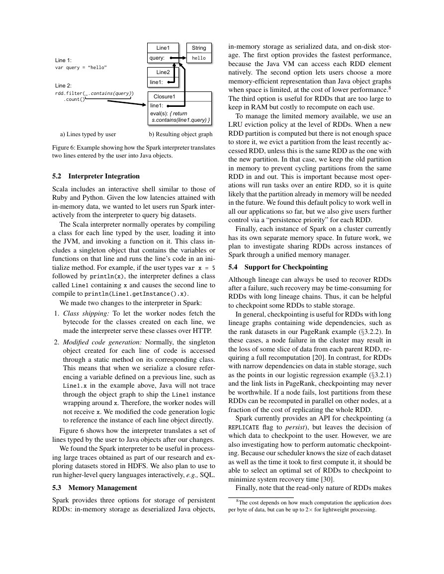
Figure 6: Example showing how the Spark interpreter translates
two lines entered by the user into Java objects.
Interpreter Integration
5.2
Scala includes an interactive shell similar to those of
Ruby and Python. Given the low latencies attained with
in-memory data, we wanted to let users run Spark inter-
actively from the interpreter to query big datasets.
The Scala interpreter normally operates by compiling
a class for each line typed by the user, loading it into
the JVM, and invoking a function on it. This class in-
cludes a singleton object that contains the variables or
functions on that line and runs the line’s code in an ini-
tialize method. For example, if the user types var x = 5
followed by println(x), the interpreter defines a class
called Line1 containing x and causes the second line to
compile to println(Line1.getInstance().x).
We made two changes to the interpreter in Spark:
1. Class shipping: To let the worker nodes fetch the
bytecode for the classes created on each line, we
made the interpreter serve these classes over HTTP.
2. Modified code generation: Normally, the singleton
object created for each line of code is accessed
through a static method on its corresponding class.
This means that when we serialize a closure refer-
encing a variable defined on a previous line, such as
Line1.x in the example above, Java will not trace
through the object graph to ship the Line1 instance
wrapping around x. Therefore, the worker nodes will
not receive x. We modified the code generation logic
to reference the instance of each line object directly.
Figure 6 shows how the interpreter translates a set of
lines typed by the user to Java objects after our changes.
We found the Spark interpreter to be useful in process-
ing large traces obtained as part of our research and ex-
ploring datasets stored in HDFS. We also plan to use to
run higher-level query languages interactively, e.g., SQL.
5.3 Memory Management
Spark provides three options for storage of persistent
RDDs: in-memory storage as deserialized Java objects,
var query = “hello” rdd.filter(_.contains(query)) .count() Line 1: Line 2: Closure1 line1: eval(s): { return s.contains(line1.query) } Line1 query: String hello Line2 line1: a) Lines typed by user b) Resulting object graph �




 2023年江西萍乡中考道德与法治真题及答案.doc
 2012年重庆南川中考生物真题及答案.doc
 2013年江西师范大学地理学综合及文艺理论基础考研真题.doc
 2020年四川甘孜小升初语文真题及答案I卷.doc
 2020年注册岩土工程师专业基础考试真题及答案.doc
 2023-2024学年福建省厦门市九年级上学期数学月考试题及答案.doc
 2021-2022学年辽宁省沈阳市大东区九年级上学期语文期末试题及答案.doc
 2022-2023学年北京东城区初三第一学期物理期末试卷及答案.doc
 2018上半年江西教师资格初中地理学科知识与教学能力真题及答案.doc
 2012年河北国家公务员申论考试真题及答案-省级.doc
 2020-2021学年江苏省扬州市江都区邵樊片九年级上学期数学第一次质量检测试题及答案.doc
 2022下半年黑龙江教师资格证中学综合素质真题及答案.doc