Implicit Active Contours Driven by Local Binary Fitting Energy
Chunming Li 1, Chiu-Yen Kao 2, John C. Gore 1, and Zhaohua Ding 1
1 Institute of Imaging Science
Vanderbilt University
2 Department of Mathematics
The Ohio State University
Nashville, TN 37232-2310, USA
{chunming.li,john.gore,zhaohua.ding}@vanderbilt.edu
Columbus, OH 43210-1174, USA
kao@math.ohio-state.edu
Abstract
Local image information is crucial for accurate segmen-
tation of images with intensity inhomogeneity. However, im-
age information in local region is not embedded in popular
region-based active contour models, such as the piecewise
constant models. In this paper, we propose a region-based
active contour model that is able to utilize image informa-
tion in local regions. The major contribution of this paper is
the introduction of a local binary fitting energy with a kernel
function, which enables the extraction of accurate local im-
age information. Therefore, our model can be used to seg-
ment images with intensity inhomogeneity, which overcomes
the limitation of piecewise constant models. Comparisons
with other major region-based models, such as the piece-
wise smooth model, show the advantages of our method in
terms of computational efficiency and accuracy.
In addi-
tion, the proposed method has promising application to im-
age denoising.
1. Introduction
Active contour models have been one of the most suc-
cessful methods for image segmentation [1, 3–7, 12]. The
existing active contour models can be categorized into two
classes: edge-based models [1, 4–6] and region-based mod-
els [2,9,10]. These two types of models both have their pros
and cons, and the choice of them in applications depends on
different characteristics of images.
Edge-based models utilize image gradient to stop the
evolving contours on the object boundaries. Typical edge-
based active contour models have an edge-based stopping
term and a balloon force term to control the motion of the
contour. The edge-based stopping term serves to stop the
contour on the desired object boundary. The balloon force
term is introduced to shrink or expand the active contour
so that the initial contour can be placed far away from the
desired object boundary. However, appropriate choice of
balloon force is sometimes difficult.
If the balloon force
is not large enough, the evolving contour may not able to
pass some narrow parts of the object. If the balloon force is
too large, the active contour is likely to pass through weak
object boundary.
Region-based active contour models have the following
advantages over edge-based models. First, region-based
models do not utilize the image gradient and therefore have
better performance for the image with weak object bound-
aries. Second, they are significantly less sensitive to the
location of initial contours. One of the most popular region-
based active contour models is Chan-Vese model [2]. This
model has been successful for images with two regions,
each having a distinct mean of pixel intensity. In [11], Vese
and Chan extended their earlier work in [2] by using a mul-
tiphase level set formulation, in which multiple regions can
be represented by multiple level set functions. These mod-
els are called piecewise constant (PC) models, since they
assume that an image consists of statistically homogeneous
regions. However, the regions of interest in images are often
not statistically homogeneous, and therefore the PC models
are not applicable to those types of images.
To handle more general scenario, Vese and Chan [11]
and Tsai et al. [10] proposed two similar region-based ac-
tive contour models, aiming at minimization of Mumford-
Shah functional [8].
In [11], Vese and Chan proposed a
piecewise smooth (PS) model, which overcomes the limita-
tion of their original work [2]. But these methods are com-
putationally inefficient. The technique proposed by Tsai et
al. [10] can address the segmentation of images with in-
tensity inhomogeneity. However, the computation in their
method is also expensive. As proposed in [10], one way to
reduce the computational cost is to use a contour near the
object boundaries as the initial contour.
In their method,
such initial contour is obtained by a preliminary segmenta-
tion using other active contour models, such as Chan and
Vese’s PC model. However, for images with intensity inho-
mogeneity, PC model can result in a contour that is still far
1
1-4244-1180-7/07/$25.00 ©2007 IEEE
�
away from the object boundary. In this situation, their two-
stage approach still cannot significantly reduce the compu-
tational cost.
In fact, intensity inhomogeneity occurs in many real im-
ages of different modalities. In particular, it is often seen
in medical images, such as X-ray radiography/tomography
and magnetic resonance (MR) images, due to technical lim-
itations or artifacts introduced by the object being imaged.
For example, intensity inhomogeneity typically appears in
MR images (see Fig. 4 for example). The inhomogeneity
in MR images arises from non-uniform magnetic field pro-
duced by radio-frequency coils as well as from object sus-
ceptibility. The degree of this inhomogeneity is worse for
higher field imaging (e.g., 7T MR) which is being increas-
ingly used in research. Therefore, overcoming the difficulty
of segmentation due to image inhomogeneity is a main mo-
tivation of this paper.
In this paper, we propose a novel active contour model
that is able to segment images with intensity inhomogene-
ity. The basic idea is to introduce a kernel function to de-
fine a local binary fitting energy in a variational formulation,
so that local intensity information can be embedded into a
region-based active contour model. The local binary fitting
energy functional is further incorporated into a variational
level set formulation without reinitialization proposed by Li
et al. [6]. Therefore, no reinitialization is necessary in the
proposed method.
2. Background
2.1. Mumford-Shah functional for image segmen-
tation
Let Ω ⊂ 2 be the image domain, and I : Ω → be a
given image. In [8], Mumford and Shah formulated image
segmentation as a problem of seeking an optimal contour C
that divides the image domain into disjoint subregions, and
an optimal function u that fits the original image I and that
is smooth within each of the subregions. They proposed the
following energy functional:
F M S(u, C) =
Ω
Ω\C
(I−u)2dxdy+ν
|∇u|2dxdy+ν|C|
(1)
where |C| is the length of contour C. Thus, image segmen-
tation can be performed by minimizing the above functional
over all the contours and fitting function u. However, it is
difficult to minimize the above functional (1), due to differ-
ent nature of the two unknowns: a contour C and a function
u, and the non-convexity of the functional as well. For prac-
tical applications, much works have been done to simplified
or modified the above Mumford-Shah functional, including
the two well known approaches that are reviewed below.
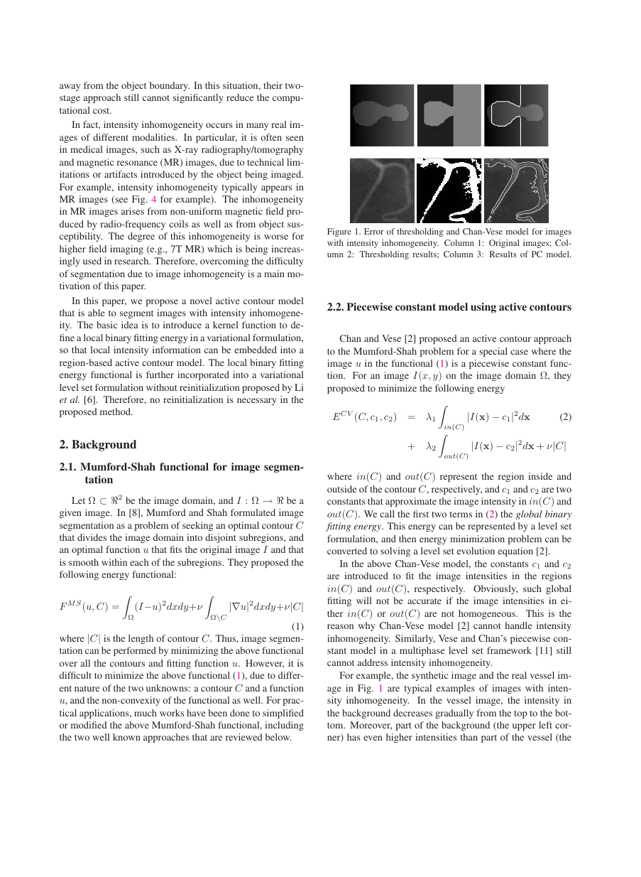
Figure 1. Error of thresholding and Chan-Vese model for images
with intensity inhomogeneity. Column 1: Original images; Col-
umn 2: Thresholding results; Column 3: Results of PC model.
2.2. Piecewise constant model using active contours
Chan and Vese [2] proposed an active contour approach
to the Mumford-Shah problem for a special case where the
image u in the functional (1) is a piecewise constant func-
tion. For an image I(x, y) on the image domain Ω, they
proposed to minimize the following energy
ECV (C, c1, c2) = λ1
+ λ2
in(C)
|I(x) − c1|2dx
(2)
|I(x) − c2|2dx + ν|C|
out(C)
where in(C) and out(C) represent the region inside and
outside of the contour C, respectively, and c1 and c2 are two
constants that approximate the image intensity in in(C) and
out(C). We call the first two terms in (2) the global binary
fitting energy. This energy can be represented by a level set
formulation, and then energy minimization problem can be
converted to solving a level set evolution equation [2].
In the above Chan-Vese model, the constants c1 and c2
are introduced to fit the image intensities in the regions
in(C) and out(C), respectively. Obviously, such global
fitting will not be accurate if the image intensities in ei-
ther in(C) or out(C) are not homogeneous. This is the
reason why Chan-Vese model [2] cannot handle intensity
inhomogeneity. Similarly, Vese and Chan’s piecewise con-
stant model in a multiphase level set framework [11] still
cannot address intensity inhomogeneity.
For example, the synthetic image and the real vessel im-
age in Fig. 1 are typical examples of images with inten-
sity inhomogeneity.
In the vessel image, the intensity in
the background decreases gradually from the top to the bot-
tom. Moreover, part of the background (the upper left cor-
ner) has even higher intensities than part of the vessel (the
�
lower left branch). The second and the third columns of
Fig. 1 show the segmentation results using thresholding and
the PC model, respectively. It is clearly seen that part of
the background is incorrectly identified as the foreground,
while part of the foreground is labeled as the background.
2.3. Piecewise smooth model and its difficulties
The PS models proposed by Vese and Chan [11] and Tsai
et al. [10] have overcome the difficulties of PC models in
the presence of image inhomogeneity. Instead of approx-
imating an image I by a piecewise constant function, the
PS model approximates the image by two smooth func-
tions u+(x) and u−(x) in the subregions Ω+ = {x ∈
Ω : φ(x) < 0} and Ω− = {x ∈ Ω : φ(x) < 0}, re-
spectively. By definition, the functions u+ and u−
are de-
fined on two exclusive subregions Ω+ and Ω−
, respectively.
However, the level set evolution equation derived to mini-
mize the energy functional in the PS model is with respect
to the level set function φ, which is defined on the full do-
main Ω. Therefore, there is an unavoidable step that extends
u+ and u−
to the full domain Ω. Moreover, the smoothness
|∇u+|2dx and µ
of the functions u+ and u−
is enforced by the smoothing
terms µ
tional in the PS model, which leads to two PDEs with the
unknown functions u+ and u−
that have to be solved at each
iteration of the level set function φ.
|∇u−|2dx in the energy func-
In addition, it is necessary to periodically reinitialize the
level set function φ to a signed distance function in practi-
cal application of the PS model. In summary, the need of
solving PDEs for u+ and u−
, the extension of u+ and u−
,
and the reinitialization makes the PS model computation-
ally very expensive. Moreover, these procedures introduce
quite a few parameters to the PS models, which increases
the difficulty of selecting parameters in using the PS model,
especially for inexperienced users.
3. Local binary fitting active contour model
and its level set formulation
3.1. Active contours with local binary fitting energy
Consider a given vector valued image I : Ω → d,
where Ω ⊂ n is the image domain, and d ≥ 1 is the
dimension of the vector I(x). For gray level images, d = 1,
for color images, d = 3. Let C be a contour in the image
domain Ω. We define for each point x ∈ Ω the following
energy
x
= λ1
E LBF
in(C)
+ λ2
out(C)
(C, f1(x), f2(x))
K(x − y)|I(y) − f1(x)|2dy
K(x − y)|I(y) − f2(x)|2dy
(3)
where λ1 and λ2 are positive constants, and K is a kernel
function with a localization property that K(u) decreases
and approaches zero as |u| increases, and f1(x) and f2(x)
are two numbers that fit image intensities near the point x.
We call the point x the center point of the above integral,
and the above energy the local binary fitting (LBF) energy
around the center point x.
In this paper, we choose the kernel function K(x) as a
Gaussian kernel
Kσ(x) =
1
(2π)n/2σn
e−|x|2/2σ2
,
(4)
with a scale parameter σ > 0. It should be emphasized that
the numbers f1 and f2 that minimize the energy (3) vary
with the center point x. The introduction of the spatially
varying fitting functions f1 and f2 makes our method es-
sentially different from piecewise constant models.
x
In the proposed model, the fitting energy in (3) is local
to the center point x in the sense that the values f1 and f2
only fit the image intensities near each x. This is due to
the kernel function K with the above localization property
that K(x − y) takes larger values at the points y near the
center point x, and it decreases to 0 as y goes away from
x. Therefore, the image intensities at the points y near the
point x have dominant influence on the values of f1 and f2
that minimize E LBF
(C, f1, f2), whereas the image intensi-
ties at the points y far away from the center point x have
almost no influence on the values of f1 and f2.
As mentioned above, the values f1 and f2 that minimize
the LBF energy E LBF
(C, f1, f2) are functions of the center
point x due to the localization property of the kernel func-
tion K(x− y). Obviously, for each center point x, the local
fitting energy E LBF
can be minimized when the contour
C is exactly on the object boundary and the fitting values
f1 and f2 are chosen optimally. However, the above en-
is defined locally for a center point x ∈ Ω. To
ergy E LBF
find the entire object boundary, we must minimize E LBF
for all the center points x in the image domain Ω. This can
be achieved by minimize the integral of E LBF
over all the
center points x in the image domain Ω. So, we define the
following energy functional
x
x
x
x
x
Ω
E(C, f1, f2) =
E LBF
x
(C, f1(x), f2(x))dx
(5)
This energy can be converted to an equivalent level set for-
mulation, from which an implicit active contour model will
be obtained to automatically handle topological changes
(see below).
3.2. Variational level set formulation of the model
In level set methods, a contour C ⊂ Ω is represented
by the zero level set of a Lipschitz function φ : Ω → .
�
the energy functional
With the level set representation,
E LBF
x
(C, f1(x), f2(x)) in (3) can be rewritten as
E LBF
(φ, f1(x), f2(x))
Kσ(x − y)|I(y) − f1(x)|2H(φ(y))dy
(6)
Kσ(x − y)|I(y) − f2(x)|2(1 − H(φ(y)))dy
x
= λ1
+ λ2
where H is the Heaviside function. Thus, the fitting energy
E in Eq. (5) can be written as
x
E LBF (φ, f1, f2)
E LBF
[
[
=
Ω
= λ1
+ λ2
(φ, f1(x), f2(x))dx
Kσ(x − y)|I(y) − f1(x)|2H(φ(y))dy]dx
Kσ(x − y)|I(y) − f2(x)|2
·(1 − H(φ(y)))dy]dx
(7)
In order to ensure stable evolution of the level set function
φ, we add the distance regularizing term in Li et al.’s vari-
ational level set formulation [6] to penalize the deviation of
the level set function φ from a signed distance function. The
deviation of the level set function φ from a signed distance
function is characterized by the following integral
P(φ) =
(|φ(x)| − 1)2dx
1
2
(8)
To regularize the zero level contour of φ, we also need the
length of the zero level curve (surface) of φ, which is given
by
L(φ) =
δ(φ(x))|φ(x)|dx
Ω
Ω
Now, we define the entire energy functional
F(φ, f1, f2) = E LBF (φ, f1, f2) + µP(φ) + νL(φ) (10)
where µ and ν are nonnegative constants.
In practice, the Heaviside function H in Eq. (6) is ap-
proximated by a smooth function Hε defined by
(9)
∂φ
∂t
and Lε. As in [2, 11], we choose ε = 1.0 for good ap-
proximation of H and δ by Hε and δε. Thus, the energy
functional F(φ, f1, f2) in (10) is approximated by
Fε(φ, f1, f2) = E LBF
(φ, f1, f2)+ µP(φ)+ νLε(φ) (13)
ε
This is the energy functional we will minimize to find the
object boundary.
3.3. Gradient descent flow
We use the standard gradient descent (or steepest de-
scent) method to minimize the energy functional (13). The
derivation of the gradient flow is similar to that of the PC
and PS models in [2,11]. The detailed procedure is given as
the following.
For a fixed level set function φ, we minimize the func-
tional Fε(φ, f1, f2) in (13) with respect to the functions
f1(x) and f2(x). By calculus of variations, it can be
shown that the functions f1(x) and f2(x) that minimize
Fε(φ, f1, f2) for a fixed function φ are given by
f1(x) = Kσ(x) ∗ [Hε(φ(x))I(x)]
Kσ(x) ∗ Hε(φ(x))
(14)
and
f2(x) = Kσ(x) ∗ [(1 − Hε(φ(x)))I(x)]
Kσ(x) ∗ [1 − Hε(φ(x))]
(15)
Note that the denominators in (14) and (15) are always pos-
itive, due to the fact that Hε(φ) > 0 and 1 − Hε(φ) > 0 by
the definition of Hε in (11).
Keeping f1 and f2 fixed, and minimizing the energy
functional Fε(φ, f1, f2) with respect to φ, we derive the
gradient descent flow:
= −δε(φ)(λ1e1 − λ2e2) + νδε(φ)div
φ
|φ|
+ µ
2φ − div
φ
|φ|
(16)
where δε is the smooth Dirac function given by (12), and e1
and e2 are the functions as below
e1(x) =
e2(x) =
Ω
Ω
Kσ(y − x)|I(x) − f1(y)|2dy
(17)
Kσ(y − x)|I(x) − f2(y)|2dy
(18)
where f1 and f2 are given by (14) and (15), respectively.
The above equation (16) is the proposed implicit active con-
tour model in this paper. We call this model LBF active
contour model to distinguish it from the PC and PS models.
Hε(x) =
1
2
[1 +
2
π
arctan( x
ε
)]
(11)
and
The derivative of Hε is the following smooth function
δε(x) = H
ε(x) =
1
π
ε
ε2 + x2
(12)
By replacing H and δ in (7) and (9) with Hε and δε, the
energy functionals E LBF and L are regularized as E LBF
ε
�
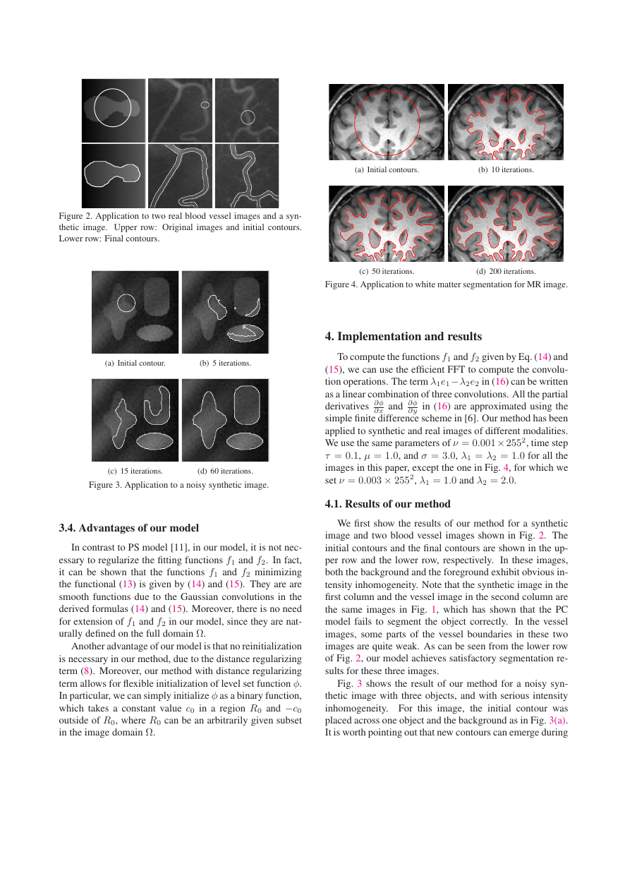
Figure 2. Application to two real blood vessel images and a syn-
thetic image. Upper row: Original images and initial contours.
Lower row: Final contours.
(a) Initial contour.
(b) 5 iterations.
(c) 15 iterations.
(d) 60 iterations.
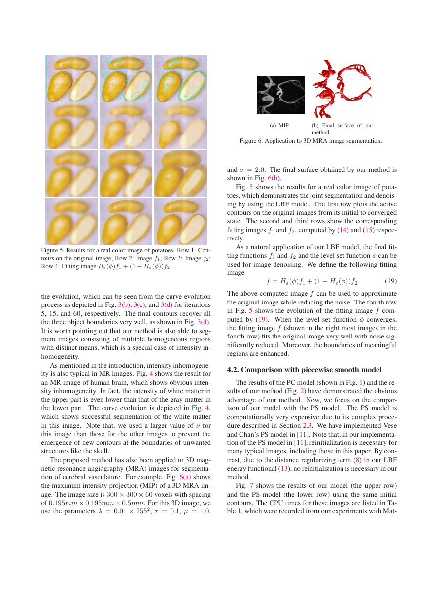
Figure 3. Application to a noisy synthetic image.
3.4. Advantages of our model
In contrast to PS model [11], in our model, it is not nec-
essary to regularize the fitting functions f1 and f2. In fact,
it can be shown that the functions f1 and f2 minimizing
the functional (13) is given by (14) and (15). They are are
smooth functions due to the Gaussian convolutions in the
derived formulas (14) and (15). Moreover, there is no need
for extension of f1 and f2 in our model, since they are nat-
urally defined on the full domain Ω.
Another advantage of our model is that no reinitialization
is necessary in our method, due to the distance regularizing
term (8). Moreover, our method with distance regularizing
term allows for flexible initialization of level set function φ.
In particular, we can simply initialize φ as a binary function,
which takes a constant value c0 in a region R0 and −c0
outside of R0, where R0 can be an arbitrarily given subset
in the image domain Ω.
(a) Initial contours.
(b) 10 iterations.
(c) 50 iterations.
(d) 200 iterations.
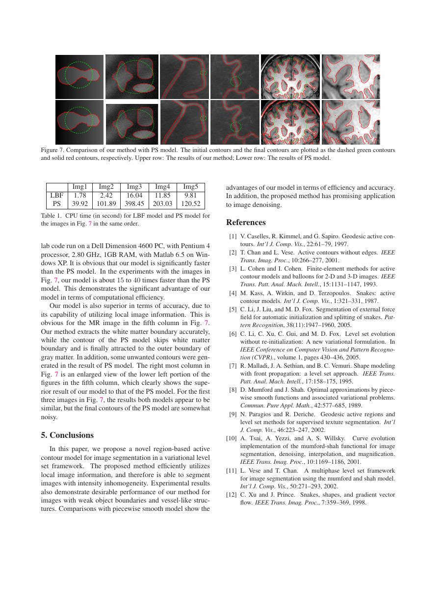
Figure 4. Application to white matter segmentation for MR image.
4. Implementation and results
∂x and ∂φ
To compute the functions f1 and f2 given by Eq. (14) and
(15), we can use the efficient FFT to compute the convolu-
tion operations. The term λ1e1−λ2e2 in (16) can be written
as a linear combination of three convolutions. All the partial
derivatives ∂φ
∂y in (16) are approximated using the
simple finite difference scheme in [6]. Our method has been
applied to synthetic and real images of different modalities.
We use the same parameters of ν = 0.001× 2552, time step
τ = 0.1, µ = 1.0, and σ = 3.0, λ1 = λ2 = 1.0 for all the
images in this paper, except the one in Fig. 4, for which we
set ν = 0.003 × 2552, λ1 = 1.0 and λ2 = 2.0.
4.1. Results of our method
We first show the results of our method for a synthetic
image and two blood vessel images shown in Fig. 2. The
initial contours and the final contours are shown in the up-
per row and the lower row, respectively. In these images,
both the background and the foreground exhibit obvious in-
tensity inhomogeneity. Note that the synthetic image in the
first column and the vessel image in the second column are
the same images in Fig. 1, which has shown that the PC
model fails to segment the object correctly. In the vessel
images, some parts of the vessel boundaries in these two
images are quite weak. As can be seen from the lower row
of Fig. 2, our model achieves satisfactory segmentation re-
sults for these three images.
Fig. 3 shows the result of our method for a noisy syn-
thetic image with three objects, and with serious intensity
inhomogeneity. For this image, the initial contour was
placed across one object and the background as in Fig. 3(a).
It is worth pointing out that new contours can emerge during
�
(a) MIP.
(b) Final surface of our
method.
Figure 6. Application to 3D MRA image segmentation.
and σ = 2.0. The final surface obtained by our method is
shown in Fig. 6(b).
Fig. 5 shows the results for a real color image of pota-
toes, which demonstrates the joint segmentation and denois-
ing by using the LBF model. The first row plots the active
contours on the original images from its initial to converged
state. The second and third rows show the corresponding
fitting images f1 and f2, computed by (14) and (15) respec-
tively.
As a natural application of our LBF model, the final fit-
ting functions f1 and f2 and the level set function φ can be
used for image denoising. We define the following fitting
image
f = Hε(φ)f1 + (1 − Hε(φ))f2
(19)
The above computed image f can be used to approximate
the original image while reducing the noise. The fourth row
in Fig. 5 shows the evolution of the fitting image f com-
puted by (19). When the level set function φ converges,
the fitting image f (shown in the right most images in the
fourth row) fits the original image very well with noise sig-
nificantly reduced. Moreover, the boundaries of meaningful
regions are enhanced.
4.2. Comparison with piecewise smooth model
The results of the PC model (shown in Fig. 1) and the re-
sults of our method (Fig. 2) have demonstrated the obvious
advantage of our method. Now, we focus on the compar-
ison of our model with the PS model. The PS model is
computationally very expensive due to its complex proce-
dure described in Section 2.3. We have implemented Vese
and Chan’s PS model in [11]. Note that, in our implementa-
tion of the PS model in [11], reinitialization is necessary for
many typical images, including those in this paper. By con-
trast, due to the distance regularizing term (8) in our LBF
energy functional (13), no reinitialization is necessary in our
method.
Fig. 7 shows the results of our model (the upper row)
and the PS model (the lower row) using the same initial
contours. The CPU times for these images are listed in Ta-
ble 1, which were recorded from our experiments with Mat-
Figure 5. Results for a real color image of potatoes. Row 1: Con-
tours on the original image; Row 2: Image f1; Row 3: Image f2;
Row 4: Fitting image Hε(φ)f1 + (1 − Hε(φ))f2.
the evolution, which can be seen from the curve evolution
process as depicted in Fig. 3(b), 3(c), and 3(d) for iterations
5, 15, and 60, respectively. The final contours recover all
the three object boundaries very well, as shown in Fig. 3(d).
It is worth pointing out that our method is also able to seg-
ment images consisting of multiple homogeneous regions
with distinct means, which is a special case of intensity in-
homogeneity.
As mentioned in the introduction, intensity inhomogene-
ity is also typical in MR images. Fig. 4 shows the result for
an MR image of human brain, which shows obvious inten-
sity inhomogeneity. In fact, the intensity of white matter in
the upper part is even lower than that of the gray matter in
the lower part. The curve evolution is depicted in Fig. 4,
which shows successful segmentation of the white matter
in this image. Note that, we used a larger value of ν for
this image than those for the other images to prevent the
emergence of new contours at the boundaries of unwanted
structures like the skull.
The proposed method has also been applied to 3D mag-
netic resonance angiography (MRA) images for segmenta-
tion of cerebral vasculature. For example, Fig. 6(a) shows
the maximum intensity projection (MIP) of a 3D MRA im-
age. The image size is 300 × 300 × 60 voxels with spacing
of 0.195mm× 0.195mm× 0.5mm. For this 3D image, we
use the parameters λ = 0.01 × 2552, τ = 0.1, µ = 1.0,
�
Figure 7. Comparison of our method with PS model. The initial contours and the final contours are plotted as the dashed green contours
and solid red contours, respectively. Upper row: The results of our method; Lower row: The results of PS model.
Img1
1.78
39.92
Img2
2.42
101.89
Img3
16.04
398.45
Img4
11.85
203.03
Img5
9.81
120.52
LBF
PS
advantages of our model in terms of efficiency and accuracy.
In addition, the proposed method has promising application
to image denoising.
Table 1. CPU time (in second) for LBF model and PS model for
the images in Fig. 7 in the same order.
References
lab code run on a Dell Dimension 4600 PC, with Pentium 4
processor, 2.80 GHz, 1GB RAM, with Matlab 6.5 on Win-
dows XP. It is obvious that our model is significantly faster
than the PS model. In the experiments with the images in
Fig. 7, our model is about 15 to 40 times faster than the PS
model. This demonstrates the significant advantage of our
model in terms of computational efficiency.
Our model is also superior in terms of accuracy, due to
its capability of utilizing local image information. This is
obvious for the MR image in the fifth column in Fig. 7.
Our method extracts the white matter boundary accurately,
while the contour of the PS model skips white matter
boundary and is finally attracted to the outer boundary of
gray matter. In addition, some unwanted contours were gen-
erated in the result of PS model. The right most column in
Fig. 7 is an enlarged view of the lower left portion of the
figures in the fifth column, which clearly shows the supe-
rior result of our model to that of the PS model. For the first
three images in Fig. 7, the results both models appear to be
similar, but the final contours of the PS model are somewhat
noisy.
5. Conclusions
In this paper, we propose a novel region-based active
contour model for image segmentation in a variational level
set framework. The proposed method efficiently utilizes
local image information, and therefore is able to segment
images with intensity inhomogeneity. Experimental results
also demonstrate desirable performance of our method for
images with weak object boundaries and vessel-like struc-
tures. Comparisons with piecewise smooth model show the
[1] V. Caselles, R. Kimmel, and G. Sapiro. Geodesic active con-
tours. Int’l J. Comp. Vis., 22:61–79, 1997.
[2] T. Chan and L. Vese. Active contours without edges. IEEE
Trans. Imag. Proc., 10:266–277, 2001.
[3] L. Cohen and I. Cohen. Finite-element methods for active
contour models and balloons for 2-D and 3-D images. IEEE
Trans. Patt. Anal. Mach. Intell., 15:1131–1147, 1993.
[4] M. Kass, A. Witkin, and D. Terzopoulos. Snakes: active
contour models. Int’l J. Comp. Vis., 1:321–331, 1987.
[5] C. Li, J. Liu, and M. D. Fox. Segmentation of external force
field for automatic initialization and splitting of snakes. Pat-
tern Recognition, 38(11):1947–1960, 2005.
[6] C. Li, C. Xu, C. Gui, and M. D. Fox. Level set evolution
without re-initialization: A new variational formulation. In
IEEE Conference on Computer Vision and Pattern Recogno-
tion (CVPR)., volume 1, pages 430–436, 2005.
[7] R. Malladi, J. A. Sethian, and B. C. Vemuri. Shape modeling
IEEE Trans.
with front propagation: a level set approach.
Patt. Anal. Mach. Intell., 17:158–175, 1995.
[8] D. Mumford and J. Shah. Optimal approximations by piece-
wise smooth functions and associated variational problems.
Commun. Pure Appl. Math., 42:577–685, 1989.
[9] N. Paragios and R. Deriche. Geodesic active regions and
level set methods for supervised texture segmentation. Int’l
J. Comp. Vis., 46:223–247, 2002.
[10] A. Tsai, A. Yezzi, and A. S. Willsky. Curve evolution
implementation of the mumford-shah functional for image
segmentation, denoising, interpolation, and magnification.
IEEE Trans. Imag. Proc., 10:1169–1186, 2001.
[11] L. Vese and T. Chan. A multiphase level set framework
for image segmentation using the mumford and shah model.
Int’l J. Comp. Vis., 50:271–293, 2002.
[12] C. Xu and J. Prince. Snakes, shapes, and gradient vector
flow. IEEE Trans. Imag. Proc., 7:359–369, 1998.
�


 2023年江西萍乡中考道德与法治真题及答案.doc
 2012年重庆南川中考生物真题及答案.doc
 2013年江西师范大学地理学综合及文艺理论基础考研真题.doc
 2020年四川甘孜小升初语文真题及答案I卷.doc
 2020年注册岩土工程师专业基础考试真题及答案.doc
 2023-2024学年福建省厦门市九年级上学期数学月考试题及答案.doc
 2021-2022学年辽宁省沈阳市大东区九年级上学期语文期末试题及答案.doc
 2022-2023学年北京东城区初三第一学期物理期末试卷及答案.doc
 2018上半年江西教师资格初中地理学科知识与教学能力真题及答案.doc
 2012年河北国家公务员申论考试真题及答案-省级.doc
 2020-2021学年江苏省扬州市江都区邵樊片九年级上学期数学第一次质量检测试题及答案.doc
 2022下半年黑龙江教师资格证中学综合素质真题及答案.doc