一份简短入门《图神经网络GNN》笔记小册.pdf-资料库

e210439c-8727-4b39-9c4d-eacca3b70b87.pdf-第1页.png

第1页 / 共7页

e210439c-8727-4b39-9c4d-eacca3b70b87.pdf-第2页.png

第2页 / 共7页

e210439c-8727-4b39-9c4d-eacca3b70b87.pdf-第3页.png

第3页 / 共7页

e210439c-8727-4b39-9c4d-eacca3b70b87.pdf-第4页.png

第4页 / 共7页

e210439c-8727-4b39-9c4d-eacca3b70b87.pdf-第5页.png

第5页 / 共7页

e210439c-8727-4b39-9c4d-eacca3b70b87.pdf-第6页.png

第6页 / 共7页

e210439c-8727-4b39-9c4d-eacca3b70b87.pdf-第7页.png

第7页 / 共7页

Graph Neural Networks - Notes Nihal V. Nayak March 2020 1 Introduction Graph Neural Networks (GNN) is a type of neural network which learns the structure of a graph. Learning graph structure allows us to represent the nodes of the graph in the euclidean space which can be useful for several downstream machine learning tasks. Recent work on GNN has shown impressive perfor- mance on link prediction, graph classiﬁcation and semi-supervised tasks (Hamil- ton et al., 2017b). Since there is a growing interest in the machine learning community to learn more about these techniques, this document provides an introduction to GNN1. The document is organized as follows: First, we introduce the basic concepts of graphs and networks. Second, we describe the major steps used in GNNs to compute node embeddings. Next, we describe three GNN techniques that are commonly mentioned in the existing literature. Finally, we include a limited survey of other notable works in the ﬁeld. 2 Basics In this section, we will review the basics of networks that will be useful to understand the forthcoming sections. Graphs consist of a set of nodes V and edges E. They are normally repre- sented with an unweighted adjacency matrix A, which consists of 1s and 0s. 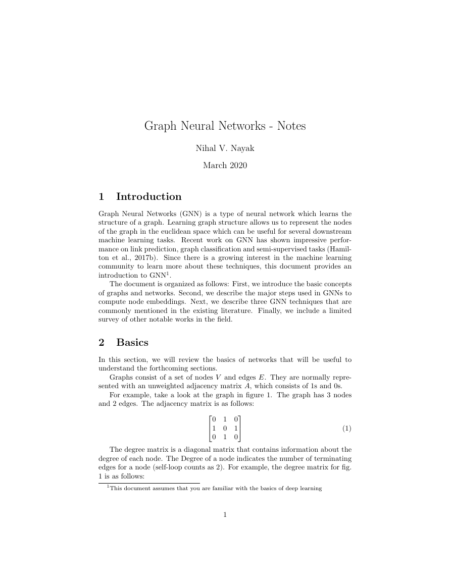For example, take a look at the graph in ﬁgure 1. The graph has 3 nodes and 2 edges. The adjacency matrix is as follows: 0 1 0  1 0 1 0 1 0 (1) The degree matrix is a diagonal matrix that contains information about the degree of each node. The Degree of a node indicates the number of terminating edges for a node (self-loop counts as 2). For example, the degree matrix for ﬁg. 1 is as follows: 1This document assumes that you are familiar with the basics of deep learning 1

1 0 0  0 2 0 0 0 1 Figure 1: Graph with 3 nodes and 2 undirected edges (2) In GNN, each node v is associated with a feature vector xv ∈ Rd. Typically, the feature vector is randomly initialized and trained on a downstream task. Although we have not introduced graph neural network, it would be useful to know how to compute the neighbors for a node. For example, from Figure 1 the neighbours of the node b are: (3) where N (.) is the neighbour function. Likewise, the neighbor of the node a N (b) = {a, c} is: N (a) = {b} (4) As you can see, each node can have a varying number of neighbors. There- fore, we need a neural network that can deal with the varying number of neigh- bors. 3 Learning on Graphs Graph Neural Network learns the structure of the graph such that the node embedding reﬂects the structure in the euclidean space (Hamilton et al., 2017b). 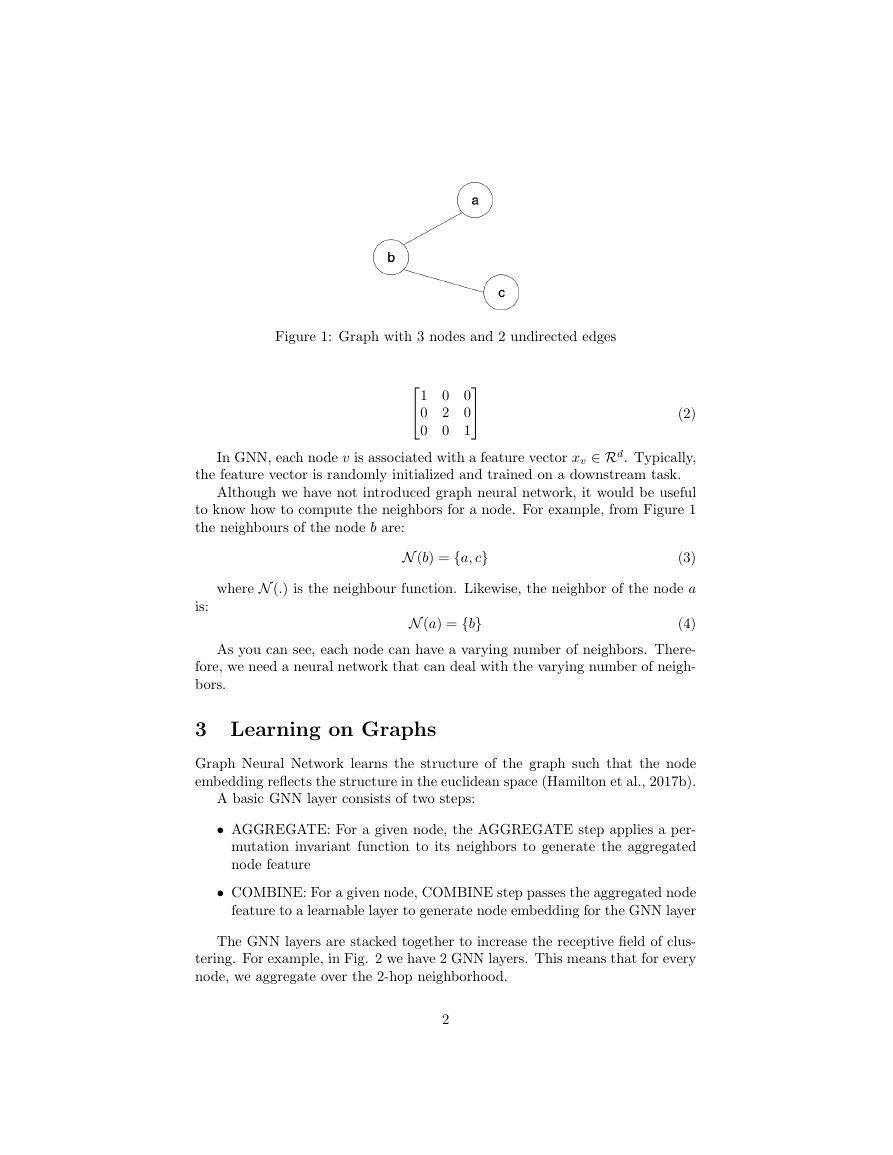A basic GNN layer consists of two steps: • AGGREGATE: For a given node, the AGGREGATE step applies a per- mutation invariant function to its neighbors to generate the aggregated node feature • COMBINE: For a given node, COMBINE step passes the aggregated node feature to a learnable layer to generate node embedding for the GNN layer The GNN layers are stacked together to increase the receptive ﬁeld of clus- tering. For example, in Fig. 2 we have 2 GNN layers. This means that for every node, we aggregate over the 2-hop neighborhood. 2

Figure 2: Left: 2 GNN layers stacked together and Right: shows the how the node feature is generated for a node (green) in a 2 layer GNN. The node (green) learns the node embedding by aggregating over 2-hop neighbourhood. AGGREGATE and COMBINE steps are sometimes called message passing phase and readout phase in the message passing neural network framework (Gilmer et al., 2017). 3.1 Formal Deﬁnition Consider the Graph G = (V, E), where V is the set of node with features Xv. There are two main steps - AGGREGATE and COMBINE at each l-th layer of the GNN: where a(l) v is the aggregated node feature of the neighbourhood, h(l−1) u node feature in neighbourhood N (.) of node v. (5) is the (6) a(l) v = AGGREGATE(l) v = COMBINE(l) h(l) h(l−1) u ∀u ∈ N (v) h(l−1) v , a(l) v where h(l) v is the node representation at the l-th iteration. h(0) v = xv where xv is the initial feature vector for the node. 4 Graph Convolutional Networks (GCN) GCN (Kipf and Welling, 2016) is a graph neural network technique that makes use of the symmetrically normalized graph laplacian2 to compute the node em- beddings. Each GCN block receives node features from the (l−1)th GCN block, i.e. the node features from the previous layer is passed to the next GCN layer, which allows for greater laplacian smoothing (Li et al., 2018). 2Refer to A for more details on Graph Laplacian. 3

4.1 Aggregate Since we don’t always have access to the entire graph structure to compute the symmetrically normalized graph laplacian, GCN Aggregator has been inter- preted as a Mean Aggregator (Xu et al., 2018a). Therefore, , u ∈ N (v) ∪ {v} a(l) v = Mean h(l−1) u (7) For each node v, the algorithm takes the mean of the neighborhood node features along with its feature (self-loop) to compute the aggregated node feature a(l) for the lth layer. This formulation makes GCN an inductive graph neural v network. 4.2 Combine The aggregated node feature a(l) v followed by a non-linear activation (ReLU) to get the node feature h(l) lth layer, is multiplied with a learnable weight matrix v for the h(l) v = ReLU W (l)a(l) v (8) where W (l) is the learnable weight matrix. 5 GraphSage Graphsage (Hamilton et al., 2017a) is a spatial graph neural network algorithm that learns node embeddings by sampling and aggregating neighbors from mul- tiple hops. Graphsage, unlike GCN, is an inductive learning algorithm which means that it does not require the entire graph structure during learning. In the original Graphsage paper, the authors describe multiple aggregators - Mean, Pooling and LSTM Aggregator. In this section, we’ll be describing the Pool Aggregator and the combine from the original paper. For simplicity, we do not sample the neighborhood nodes as well. 5.1 Aggregate Graphsage makes use of a max-pooling aggregator to compute an aggregated node feature. All the neighborhood node features are passed through a lin- ear layer. We then pass these features through a non-linear activation before applying max ﬁlter. Formally, W (l−1) pool h(l−1) u σ a(l) v = max is the aggregated node feature for the lth layer. W (l−1) + b , u ∈ N (v) (9) pool and b are where a(l) v the learnable parameters. 4

5.2 Combine The combine function concatenates the (l − 1)th layer node feature h(l−1) the aggregated feature vector a(l) neural network: with v and pass the vector through a fully connected v h(l) v = ReLU W (l)[h(l−1) v , a(l) v ] (10) where W (l) is a learnable weight matrix for lth layer. 6 Graph Attention Network (GAT) Graph Attention Network (Veliˇckovi´c et al., 2018) is a spatial graph neural network technique that uses Self Attention to aggregate the neighborhood node features. Self Attention is equivalent to computing a weighted mean of the neighbourhood node features. The original paper uses K masked self attention modules to aggregate node features. For simplicity, we consider only one self attention block. 6.1 Aggregate GAT uses an Attention module to compute the weighted mean of the neighbor- hood node features as follows: , u ∈ N (v) ∪ {v} a(l) v = Attention h(l−1) u (11) The authors use self-attention (Bahdanau et al., 2014) but the aggregation technique is agnostic to the choice attention mechanism. 6.2 Combine The aggregated node feature a(l) v followed by a non-linear activation to get the node feature h(l) is multiplied with a learnable weight matrix v for the lth layer, h(l) v = LeakyReLU W (l)a(l) v (12) where W (l) is the learnable weight matrix. 7 Related Works Apart from GCN, Graphsage, and GAT, there are few more works that fre- quently appear in the literature. SGN (Wu et al., 2019) simpliﬁes GCN by removing non-linearity between the GCN layers. Furthermore, to achieve the same “receptive ﬁeld” of having K GCN layers, they take the graph laplacian to the power of K and show equivalent performance. Xu et al. (2018b) intro- duced jumping knowledge networks that aggregate node features generated from 5

all the previous layers to compute the ﬁnal vector using mean or max-pooling. This allows the model to learn better structure-aware representations from dif- ferent neighborhood aggregations. The works described so far have not taken advantage of the relations in the graph. R-GCN (Schlichtkrull et al., 2018) and Directed-GCN (Marcheggiani and Titov, 2017) extend GCN to relational graphs. References Bahdanau, D., Cho, K., and Bengio, Y. (2014). Neural machine translation by jointly learning to align and translate. arXiv preprint arXiv:1409.0473. Gilmer, J., Schoenholz, S. S., Riley, P. F., Vinyals, O., and Dahl, G. E. (2017). Neural message passing for quantum chemistry. In Proceedings of the 34th International Conference on Machine Learning-Volume 70, pages 1263–1272. JMLR. org. Hamilton, W., Ying, Z., and Leskovec, J. (2017a). Inductive representation learning on large graphs. In Advances in Neural Information Processing Sys- tems, pages 1024–1034. Hamilton, W. L., Ying, R., and Leskovec, J. (2017b). Representation learning on graphs: Methods and applications. IEEE Data Eng. Bull., 40:52–74. Kipf, T. N. and Welling, M. (2016). Semi-supervised classiﬁcation with graph convolutional networks. Li, Q., Han, Z., and Wu, X.-M. (2018). Deeper insights into graph convolutional networks for semi-supervised learning. In Thirty-Second AAAI Conference on Artiﬁcial Intelligence. Marcheggiani, D. and Titov, I. (2017). Encoding sentences with graph convolu- tional networks for semantic role labeling. arXiv preprint arXiv:1703.04826. Schlichtkrull, M., Kipf, T. N., Bloem, P., Van Den Berg, R., Titov, I., and Welling, M. (2018). Modeling relational data with graph convolutional net- works. In European Semantic Web Conference, pages 593–607. Springer. Veliˇckovi´c, P., Cucurull, G., Casanova, A., Romero, A., Li`o, P., and Bengio, Y. (2018). Graph Attention Networks. International Conference on Learning Representations. Wu, F., Souza, A., Zhang, T., Fifty, C., Yu, T., and Weinberger, K. (2019). In International Conference on Simplifying graph convolutional networks. Machine Learning, pages 6861–6871. Xu, K., Hu, W., Leskovec, J., and Jegelka, S. (2018a). How powerful are graph neural networks? 6

Xu, K., Li, C., Tian, Y., Sonobe, T., Kawarabayashi, K.-i., and Jegelka, S. (2018b). Representation learning on graphs with jumping knowledge net- works. arXiv preprint arXiv:1806.03536. A Graph Laplacian The adjacency matrix and degree matrix can be combined to get the Graph Laplacian (commonly occurs in the literature). L = D − A (13) where L is the graph laplacian, D is the degree matrix and A is the adjacency matrix. The symmetric normalized graph laplacian can be formally deﬁned as: Lsym = D− 1 2 LD− 1 2 = I − D− 1 2 AD− 1 2 where I is the Identity matrix. The elements of Lsym are given by:  Lij = deg(vi)deg(vj) 1 1 − 0 if i == j and deg(vi) = 0 if i = j otherwise (14) (15) (16) B Original GCN In section 4, we interpreted GCN (Kipf and Welling, 2016) as a mean aggregator. However, there is a subtle diﬀerence between our interpretation and the original GCN. Consider the adjacency matrix A and its degree matrix D. Let H (l) be the node features for the lth layer and H (0) = X. The propagation rule for each GCN layer is as follows: ˜D− 1 2 H (l)W (l) f (H (l), ˜A) = σ 2 ˜A ˜D− 1 with ˜A = I + A where I is the identity matrix and degree matrix ˜D of ˜A. 7

资料库

一份简短入门《图神经网络GNN》笔记小册.pdf

相关推荐

人工智能

热门标签

最新资料