Zhang et al. Robot. Biomim. (2018) 5:3
https://doi.org/10.1186/s40638-018-0085-7
RESEARCH
A 6-DOF robot-time optimal trajectory
planning based on an improved genetic
algorithm
Jiayan Zhang, Qingxi Meng*
, Xugang Feng and Hao Shen
Open Access
Abstract
By using quintic polynomial function to interpolate several given points of each joint of the robot, the mathematical
expressions of each joint variable of the robot with time are established. In addition, to improve the search algo-
rithm performance crossover operator and mutation operator of the genetic algorithm are improved in cosine form.
Furthermore, the improved adaptive genetic algorithm is applied to optimize the time interval of interpolation points
of each joint, so as to realize time optimal trajectory planning. Moreover, MATLAB simulation is carried out, and the
results show that the method proposed in this paper reduces the running time of the robot tasks. Meanwhile, the
curves of angle position, velocity and acceleration of each joint are smooth enough, which ensure accomplish its
tasks in a stable and efficient way.
Keywords: Industrial robot, Trajectory planning, Adaptive genetic algorithm (AGA), Time optimal
Background
Robot trajectory planning usually refers to track points
given several expectations and target pose, and timely
adjust the rotation angle of each joint of the robot to the
end effector at a prescribed trajectory followed by each
point to eventually reach the target point. The trajectory
planning in joint space is simpler and convenient than
that of Cartesian space. Therefore, several fixed points
which located at the end of several robotic arms are usu-
ally given. Then, these track points for the robot are com-
puted by using the inverse kinematics so as to convert it
from Cartesian space to joint coordinate space. Next, the
track points are used to carry out interpolation opera-
tion using various spline functions, polynomial functions
or other forms of curves, and the expressions about the
time of each joint variable for the robot are obtained. In
addition, in light of the mechanical characteristics of the
robot, the speed and acceleration of each joint should be
limited to the allowable range. Therefore, it is necessary
to optimize the speed and acceleration of each joint arm,
*Correspondence: mqx3021@qq.com
College of Electrical Engineering and Information, Anhui University
of Technology, Ma’anshan 243002, China
not only to ensure the smooth operation of the joint arm
but also to reduce the wear and impact to prolong the
working life of the robot.
The method of optimal trajectory planning generally
includes time optimal trajectory planning [1–3], energy
minimum trajectory planning [3, 4] and impact mini-
mum trajectory planning [5], or multi-objective trajec-
tory optimization combining these estimation schemes.
Among them, the optimal trajectory planning with the
robot running time as main consideration is favored by
many scholars. In recent years, many researchers have
made some achievements in the field of robot trajectory
planning. Tohfeh and Fakharian [6] constructed a func-
tion expression for the omnidirectional robot’s energy
dissipation by combining obstacle avoidance perfor-
mance, and the optimization problem was transformed
into a parameter minimization problem by the poly-
nomial interpolation method, which provided a more
effective way for the study of robot obstacle avoidance.
However, due to the complexity of this method, there is a
certain degree of difficulty in practice. Bende [7] studied
a method of modeling underwater robot based on bond
graph theory and optimized the model parameters with
the genetic algorithm to obtain the optimized trajectory
© The Author(s) 2018. This article is distributed under the terms of the Creative Commons Attribution 4.0 International License
(http://creat iveco mmons .org/licen ses/by/4.0/), which permits unrestricted use, distribution, and reproduction in any medium,
provided you give appropriate credit to the original author(s) and the source, provide a link to the Creative Commons license,
and indicate if changes were made.
�
Zhang et al. Robot. Biomim. (2018) 5:3
Page 2 of 7
of the robot. Experiments were carried to show the sig-
nificance of this method. Zhu and Liu [8] applied the
seventh-order B-spline curve for the interpolation opera-
tion of robot’s articulation arm trajectory and applied
the sequential quadratic programming for the trajectory
planning, which achieved the optimal planning goal and
the angular displacement, velocity and acceleration curve
of each joint of the robot are smoother.
In this paper, from the point of view of robot run-
ning time, the trajectory of robot joint is planned by the
quintic polynomial interpolation under the premise of
smooth operation of the manipulator, and the time inter-
val of trajectory interpolation point is optimized by the
improved adaptive genetic algorithm, so that the robot
accomplishes task time as short as possible.
Model
In this paper, we consider PUMA560 robot as the
research object, which belongs to a conventional six-
arm-type robot. Its first three joints are used to deter-
mine the position of the robot end effector, and the latter
three joints are used to determine its attitude. In order
to make it easier to analyze the motion of articulation
arm of the robot, it is necessary to establish the kinematic
equation of the robot. The link pole coordinate system is
established by D-H method, and through the translation,
rotation and other coordinate transformation to establish
the relationship between the coordinate system. The link
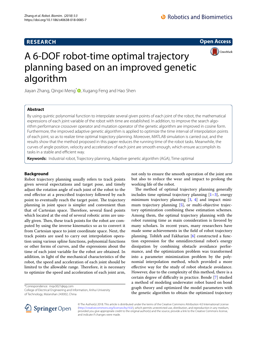
pole coordinate system is shown in Fig. 1.
0T1 =
2T3 =
4T5 =
1T2 =
3T4 =
5T6 =
cθ4 −sθ4 0 a3
1 d4
0
−sθ4 −cθ4 0 0
0 1
cθ2 −sθ2 0 0
1 d2
0
−sθ2 −cθ1 0 0
0 1
cθ6 −sθ6 0 0
0
1 0
−sθ6 −cθ6 0 0
0 1
cθ5 −sθ5 0 0
0 −1 0
0
sθ5
cθ5
0 0
0
0
0 1
cθ3 −sθ3 0 a2
cθ3 0 0
sθ3
1 0
0
0
0
0
0 1
cθ1 −sθ1 0 0
cθ1 0 0
sθ1
1 0
0
0
0
0
0 1
0
0
0
0
0
0
0
0
0
(1)
z0 (z1)
�1
x0
d2
z2
a2
x3
�2
x2
a3
y0 (x1)
6
6
0
.
4
�3
�4
d4
z3
x4 (x5)(x6)
z5
�5
z4 (z6)
o(y)
56.25
�6
n(x)
a(z)
Fig. 1 The link pole coordinate system of PUMA560 robot according
to the link pole coordinate system of Fig. 1, the transformation matrix
of each link can be obtained as follows
nx ox ax
ny oy ay
nz oz az
the posture of the end effector relative to the base system
where the third-order sub-matrix
represents
represents its position relative to the base
{0}, and
px
py
pz
system {0}.
Trajectory planning analysis
The number of desired track points of the robot end
effector in the Cartesian space is transformed into the
corresponding joint variables by the kinematic inverse
operation, and then, track points of the joint space are
interpolated to obtain the joint variables of the robot a
function of time-varying expression [9]. In this paper,
the quintic polynomial is used to interpolate trajectory
points in the robot joint space.
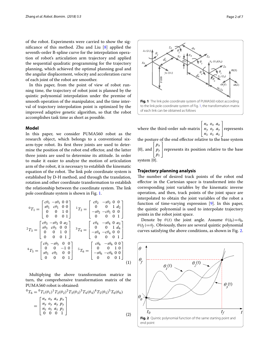
Denote by θ (t) the joint angle. Assume θ (t0) = θ0 ,
θ (tf ) = θf . Obviously, there are several quintic polynomial
curves satisfying the above conditions, as shown in Fig. 2.
Multiplying the above transformation matrice
in
turn, the comprehensive transformation matrix of the
PUMA560 robot is obtained:
0T6 = 0T1(θ 1)1T2(θ 2)2T3(θ 3)3T4(θ 4)4T5(θ 5)5T6(θ 6)
nx ox ax px
ny oy ay py
nz oz az pz
0 0 0 1
=
(2)
Fig. 2 Quintic polynomial function of the same starting point and
end point
�
Zhang et al. Robot. Biomim. (2018) 5:3
Page 3 of 7
It is now necessary to find a smooth curve with starting
point θ0 and ending point θf . In addition, the expression
of the quintic polynomial is:
θ (t) = a0 + a1t + a2t2 + a3t3 + a4t4 + a5t5
(3)
At the start and the end points, the displacement con-
straint, speed constraint and acceleration constraint are
expressed in (4)–(6), respectively:
θ (tf ) = θf
θ (0) = θ0
θ ′(0) = θ ′
θ ′′(0) = θ ′′
0
θ ′(tf ) = θ ′
f
0
θ ′′(tf ) = θ ′′
f
(4)
(5)
(6)
Deriving Eq. (3), the velocity expression of the robot’s
trajectory is obtained as:
θ ′(t) = a1 + 2a2t + 3a3t2 + 4a4t3 + 5a5t4
(7)
Similarly, by means of the second derivative of t in
formula Eq. (6), we can get the acceleration function as
follows:
θ ′′(t) = 2a2 + 6a3t + 12a4t2 + 20a5t3
(8)
Combining Eqs. (4), (5) and (6), we obtain the coeffi-
cients of the quintic polynomial as follows:
a0 = θ0
a1 = θ ′
0
θ ′′
0
a2 =
2
20θf −20θ0−(12θ ′
a3 =
a4 =
a5 =
)tf −(3θ ′′
0 −θ ′′
f
)t2
f
0+8θ ′
f
2t3
f
0+14θ ′
f
30θf −30θ0+(16θ ′
)tf +(3θ ′′
0 −2θ ′′
f
)t2
f
12θf −12θ0−(6θ ′
)tf −(θ ′′
0 −θ ′′
f
)t2
f
2t4
f
0+6θ ′
f
2t5
f
(9)
Introducing the above factors into Eq. (3), the robot
trajectory equation of the quintic polynomial can be
derived.
Improvement in genetic algorithm
The basic knowledge of the kinematics of the robot and
the basic principle of the interpolation of the trajec-
tory points of the joint space by the quintic polynomial
have been introduced in the preceding narrative. On
this basis, it is necessary to optimize the time interval
of the interpolation point of the track point by using the
genetic algorithm to realize the optimal planning of the
robot time and further make the angular displacement,
velocity and acceleration curve of each joint movement
smoother.
The genetic algorithm, which is an artificial intelligence
optimization algorithm for simulating the genetic and
evolutionary processes in nature [10–12], owns the char-
acteristics of simplicity and robustness, and starts from
the parallel solution of the problem (rather than a single
solution). Therefore, it not only has excellent global opti-
mization but also is used in the optimization process of
practical problems [13].
However, the crossover operator and mutation opera-
tor of a simple genetic algorithm are invariant in the pro-
cess of algorithm implementation and do not satisfy the
dynamic requirement of biological evolution. To this end,
Ren and San [14] proposed an adaptive genetic algorithm
according to the individual fitness of different dynamic
adjustment of crossover probability and mutation prob-
ability. The adjustment of the crossover and mutation
probabilities is shown in Eqs. (10) and (11), respectively:
pc = pc1 −
pc1,
(pc1−pc2)(f ′−favg)
fmax −favg
, f ′ ≥ favg
f ′ < favg
pm = pm1 −
pm1,
(pm1−pm2)(f ′−favg)
fmax −favg
, f ≥ favg
f ′ < favg
(10)
(11)
where pc1 = 0.9 , pc2 = 0.6 , pm1 = 0.1 , pm2 = 0.01 f ′ is
the parent of the larger fitness value; favg is the average
fitness value in the population; fmax is the fitness value of
the largest individual in the current population.
Equation (10) shows that a larger fixed crossover prob-
ability is given when the fitness value of the cross parent
is small. And the greater the fitness of the two chro-
mosomes, the smaller the crossover probability is. The
adjustment of the mutation probability in Eq. (11) is con-
sistent with the crossover probability.
It is noted that the above method has two drawbacks.
Firstly, the crossover probability and the mutation prob-
ability are fixed for the parent chromosomes whose fit-
ness is lower than the average fitness of the population.
Secondly, the adjustment of crossover and mutation
probability is linear, and it can not meet the objective of
population evolution. To overcome the two drawbacks,
this paper presents an adaptive genetic algorithm that
uses a cosine function to adjust crossover probability
and mutation probability. Adjusting Eqs. (10) and (11) as
follows:
pc0+pc min
2
pc0+pc max
2
pc =
+ pc0−pc min
+ pc0−pc max
2
2
fmax −favg
π�, f ≥ favg
cos� f −favg
cos� favg−f
π�,
f < favg
favg
(12)
�
Zhang et al. Robot. Biomim. (2018) 5:3
Page 4 of 7
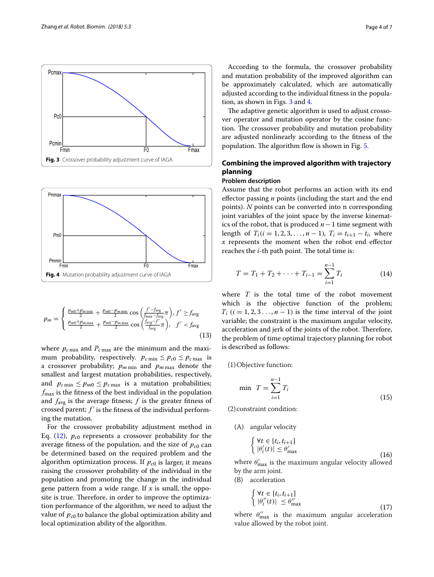
Fig. 4 Mutation probability adjustment curve of IAGA
T = T1 + T2 + · · · +T i−1 =
Pcmax
Pc0
Pcmin
Fmin
F0
Fmax
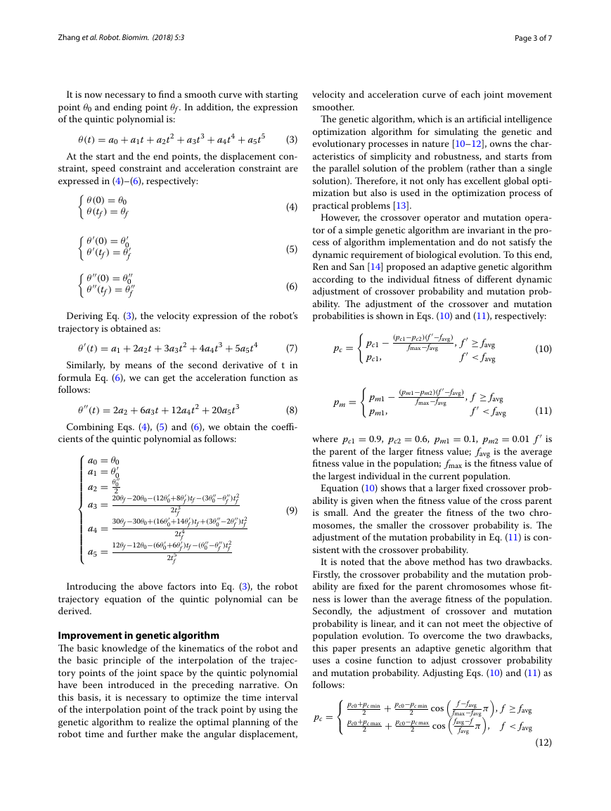
Fig. 3 Crossover probability adjustment curve of IAGA
Pmmax
Pm0
Pmmin
Fmin
F0
Fmax
pm =
pm0+pm min
2
pm0+pm max
2
+ pm0−pm min
2
+ pm0−pm max
2
fmax −favg
cos� f ′−favg
π�, f ′ ≥ favg
cos� favg−f ′
π�,
f ′ < favg
favg
(13)
where pc min and Pc max are the minimum and the maxi-
mum probability, respectively. pc min ≤ pc0 ≤ pc max is
a crossover probability; pm min and pm max denote the
smallest and largest mutation probabilities, respectively,
and pc min ≤ pm0 ≤ pc max is a mutation probabilities;
fmax is the fitness of the best individual in the population
and favg is the average fitness; f is the greater fitness of
crossed parent; f ′ is the fitness of the individual perform-
ing the mutation.
For the crossover probability adjustment method in
Eq. (12), pc0 represents a crossover probability for the
average fitness of the population, and the size of pc0 can
be determined based on the required problem and the
algorithm optimization process. If pc0 is larger, it means
raising the crossover probability of the individual in the
population and promoting the change in the individual
gene pattern from a wide range. If x is small, the oppo-
site is true. Therefore, in order to improve the optimiza-
tion performance of the algorithm, we need to adjust the
value of pc0 to balance the global optimization ability and
local optimization ability of the algorithm.
According to the formula, the crossover probability
and mutation probability of the improved algorithm can
be approximately calculated, which are automatically
adjusted according to the individual fitness in the popula-
tion, as shown in Figs. 3 and 4.
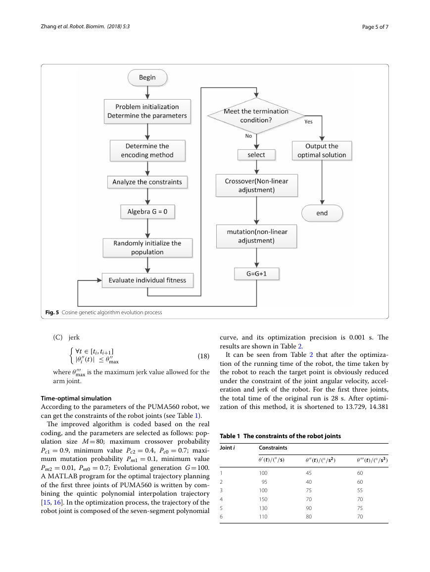
The adaptive genetic algorithm is used to adjust crosso-
ver operator and mutation operator by the cosine func-
tion. The crossover probability and mutation probability
are adjusted nonlinearly according to the fitness of the
population. The algorithm flow is shown in Fig. 5.
Combining the improved algorithm with trajectory
planning
Problem description
Assume that the robot performs an action with its end
effector passing n points (including the start and the end
points). N points can be converted into n corresponding
joint variables of the joint space by the inverse kinemat-
ics of the robot, that is produced n − 1 time segment with
length of Ti(i = 1, 2, 3, . . . , n − 1) , Ti = ti+1 − ti , where
x represents the moment when the robot end effector
reaches the i-th path point. The total time is:
Ti
n−1
i=1
(14)
is the objective
where T is the total time of the robot movement
which
function of the problem;
Ti (i = 1, 2, 3 . . . , n − 1) is the time interval of the joint
variable; the constraint is the maximum angular velocity,
acceleration and jerk of the joints of the robot. Therefore,
the problem of time optimal trajectory planning for robot
is described as follows:
(1) Objective function:
min T =
n−1
i=1
(2) constraint condition:
Ti
(15)
(A) angular velocity
∀t ∈ [ti, ti+1]
|θ ′
where θ ′
by the arm joint.
(B) acceleration
i (t)| ≤ θ ′
(16)
max is the maximum angular velocity allowed
max
∀t ∈ [ti, ti+1]
|θ ′′
i (t)| ≤ θ ′′
(17)
max is the maximum angular acceleration
max
where θ ′′
value allowed by the robot joint.
�
Zhang et al. Robot. Biomim. (2018) 5:3
Page 5 of 7
Fig. 5 Cosine genetic algorithm evolution process
(C)
jerk
∀t ∈ [ti, ti+1]
|θ ′′
where θ ′′′
arm joint.
i (t)| ≤ θ ′′
max is the maximum jerk value allowed for the
max
(18)
Time‑optimal simulation
According to the parameters of the PUMA560 robot, we
can get the constraints of the robot joints (see Table 1).
The improved algorithm is coded based on the real
coding, and the parameters are selected as follows: pop-
ulation size M = 80; maximum crossover probability
Pc1 = 0.9 , minimum value Pc2 = 0.4 , Pc0 = 0.7 ; maxi-
mum mutation probability Pm1 = 0.1 , minimum value
Pm2 = 0.01 , Pm0 = 0.7 ; Evolutional generation G = 100.
A MATLAB program for the optimal trajectory planning
of the first three joints of PUMA560 is written by com-
bining the quintic polynomial interpolation trajectory
[15, 16]. In the optimization process, the trajectory of the
robot joint is composed of the seven-segment polynomial
curve, and its optimization precision is 0.001 s. The
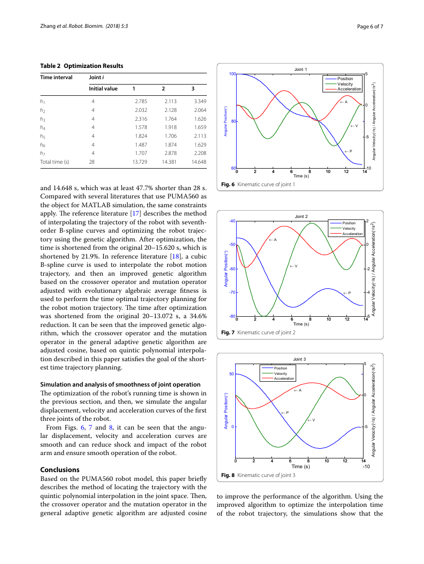
results are shown in Table 2.
It can be seen from Table 2 that after the optimiza-
tion of the running time of the robot, the time taken by
the robot to reach the target point is obviously reduced
under the constraint of the joint angular velocity, accel-
eration and jerk of the robot. For the first three joints,
the total time of the original run is 28 s. After optimi-
zation of this method, it is shortened to 13.729, 14.381
Table 1 The constraints of the robot joints
Joint i
Constraints
θ ′(t)/(◦/s)
θ ′′(t)/(◦/s2)
θ ′′′(t)/(◦/s3)
1
2
3
4
5
6
100
95
100
150
130
110
45
40
75
70
90
80
60
60
55
70
75
70
�
Zhang et al. Robot. Biomim. (2018) 5:3
Page 6 of 7
Table 2 Optimization Results
Time interval
Joint i
Initial value
1
h1
h2
h3
h4
h5
h6
h7
Total time (s)
4
4
4
4
4
4
4
28
2.785
2.032
2.316
1.578
1.824
1.487
1.707
13.729
100
)
°
(
n
o
i
t
i
s
o
P
l
r
a
u
g
n
A
80
2
2.113
2.128
1.764
1.918
1.706
1.874
2.878
14.381
3
3.349
2.064
1.626
1.659
2.113
1.629
2.208
14.648
Joint 1
5
0
-5
Position
Velocity
Acceleration
← A
← V
← P
)
2
s
/
°
(
n
o
i
t
l
a
r
e
e
c
c
A
l
r
a
u
g
n
A
/
)
s
/
°
(
y
t
i
l
c
o
e
V
l
r
a
u
g
n
A
60
0
0
2
2
4
4
6
6
8
8
Time (s)
10
10
12
12
-10
14
14
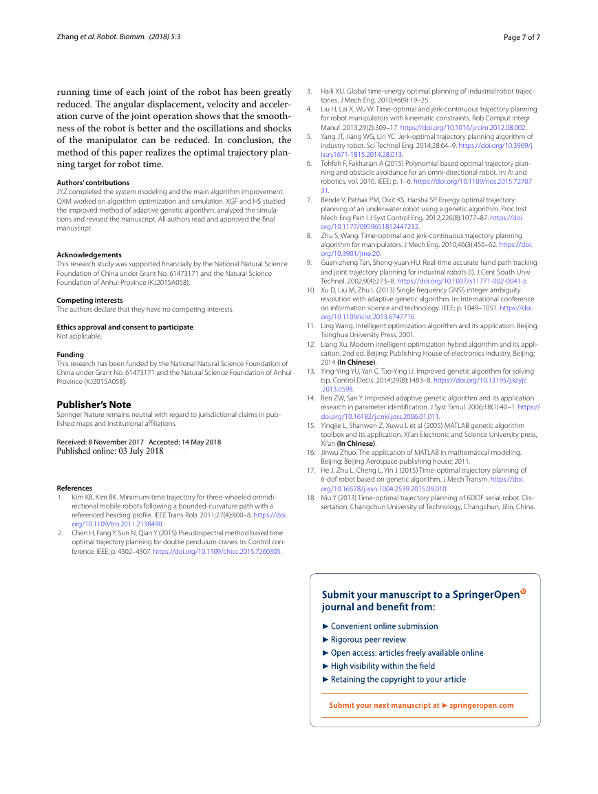
Fig. 6 Kinematic curve of joint 1
and 14.648 s, which was at least 47.7% shorter than 28 s.
Compared with several literatures that use PUMA560 as
the object for MATLAB simulation, the same constraints
apply. The reference literature [17] describes the method
of interpolating the trajectory of the robot with seventh-
order B-spline curves and optimizing the robot trajec-
tory using the genetic algorithm. After optimization, the
time is shortened from the original 20–15.620 s, which is
shortened by 21.9%. In reference literature [18], a cubic
B-spline curve is used to interpolate the robot motion
trajectory, and then an improved genetic algorithm
based on the crossover operator and mutation operator
adjusted with evolutionary algebraic average fitness is
used to perform the time optimal trajectory planning for
the robot motion trajectory. The time after optimization
was shortened from the original 20–13.072 s, a 34.6%
reduction. It can be seen that the improved genetic algo-
rithm, which the crossover operator and the mutation
operator in the general adaptive genetic algorithm are
adjusted cosine, based on quintic polynomial interpola-
tion described in this paper satisfies the goal of the short-
est time trajectory planning.
Simulation and analysis of smoothness of joint operation
The optimization of the robot’s running time is shown in
the previous section, and then, we simulate the angular
displacement, velocity and acceleration curves of the first
three joints of the robot.
From Figs. 6, 7 and 8, it can be seen that the angu-
lar displacement, velocity and acceleration curves are
smooth and can reduce shock and impact of the robot
arm and ensure smooth operation of the robot.
Conclusions
Based on the PUMA560 robot model, this paper briefly
describes the method of locating the trajectory with the
quintic polynomial interpolation in the joint space. Then,
the crossover operator and the mutation operator in the
general adaptive genetic algorithm are adjusted cosine
Joint 2
← A
← V
-40
-50
-60
-70
)
°
(
n
o
i
t
i
s
o
P
l
r
a
u
g
n
A
Joint 3
Position
Velocity
Acceleration
← A
← P
← V
50
)
°
(
n
o
i
t
i
s
o
P
l
r
a
u
g
n
A
0
Position
Velocity
Acceleration
2
0
)
2
s
/
°
(
n
o
i
t
a
r
e
e
c
c
A
l
-2
-4
← P
l
r
a
u
g
n
A
/
)
s
/
°
(
y
t
i
l
c
o
e
V
l
r
a
u
g
n
A
5
0
-5
)
2
s
/
°
(
n
o
i
t
a
r
e
e
c
c
A
l
l
r
a
u
g
n
A
/
)
s
/
°
(
y
t
i
l
c
o
e
V
l
r
a
u
g
n
A
-80
0
0
2
2
4
4
6
6
8
8
Time (s)
10
10
12
12
-6
14
14
Fig. 7 Kinematic curve of joint 2
0
0
2
2
4
4
6
6
8
8
Time (s)
10
10
12
12
14
14
-10
Fig. 8 Kinematic curve of joint 3
to improve the performance of the algorithm. Using the
improved algorithm to optimize the interpolation time
of the robot trajectory, the simulations show that the
�
Zhang et al. Robot. Biomim. (2018) 5:3
Page 7 of 7
running time of each joint of the robot has been greatly
reduced. The angular displacement, velocity and acceler-
ation curve of the joint operation shows that the smooth-
ness of the robot is better and the oscillations and shocks
of the manipulator can be reduced. In conclusion, the
method of this paper realizes the optimal trajectory plan-
ning target for robot time.
Authors’ contributions
JYZ completed the system modeling and the main algorithm improvement.
QXM worked on algorithm optimization and simulation. XGF and HS studied
the improved method of adaptive genetic algorithm, analyzed the simula-
tions and revised the manuscript. All authors read and approved the final
manuscript.
Acknowledgements
This research study was supported financially by the National Natural Science
Foundation of China under Grant No. 61473171 and the Natural Science
Foundation of Anhui Province (KJ2015A058).
Competing interests
The authors declare that they have no competing interests.
Ethics approval and consent to participate
Not applicable.
Funding
This research has been funded by the National Natural Science Foundation of
China under Grant No. 61473171 and the Natural Science Foundation of Anhui
Province (KJ2015A058).
Publisher’s Note
Springer Nature remains neutral with regard to jurisdictional claims in pub-
lished maps and institutional affiliations.
Received: 8 November 2017 Accepted: 14 May 2018
References
1. Kim KB, Kim BK. Minimum-time trajectory for three-wheeled omnidi-
rectional mobile robots following a bounded-curvature path with a
referenced heading profile. IEEE Trans Rob. 2011;27(4):800–8. https ://doi.
org/10.1109/tro.2011.21384 90.
2. Chen H, Fang Y, Sun N, Qian Y (2015) Pseudospectral method based time
optimal trajectory planning for double pendulum cranes. In: Control con-
ference. IEEE; p. 4302–4307. https ://doi.org/10.1109/chicc .2015.72603 05.
3. Haili XU. Global time-energy optimal planning of industrial robot trajec-
4.
tories. J Mech Eng. 2010;46(9):19–25.
Liu H, Lai X, Wu W. Time-optimal and jerk-continuous trajectory planning
for robot manipulators with kinematic constraints. Rob Comput Integr
Manuf. 2013;29(2):309–17. https ://doi.org/10.1016/j.rcim.2012.08.002.
5. Yang JT, Jiang WG, Lin YC. Jerk-optimal trajectory planning algorithm of
industry robot. Sci Technol Eng. 2014;28:64–9. https ://doi.org/10.3969/j.
issn.1671-1815.2014.28.013.
Tohfeh F, Fakharian A (2015) Polynomial based optimal trajectory plan-
ning and obstacle avoidance for an omni-directional robot. In: Ai and
robotics, vol. 2010. IEEE; p. 1–6. https ://doi.org/10.1109/rios.2015.72707
31.
6.
7. Bende V, Pathak PM, Dixit KS, Harsha SP. Energy optimal trajectory
planning of an underwater robot using a genetic algorithm. Proc Inst
Mech Eng Part I J Syst Control Eng. 2012;226(8):1077–87. https ://doi.
org/10.1177/09596 51812 44723 2.
8. Zhu S, Wang. Time-optimal and jerk-continuous trajectory planning
algorithm for manipulators. J Mech Eng. 2010;46(3):456–62. https ://doi.
org/10.3901/jme.20.
9. Guan-zheng Tan, Sheng-yuan HU. Real-time accurate hand path tracking
and joint trajectory planning for industrial robots (I). J Cent South Univ
Technol. 2002;9(4):273–8. https ://doi.org/10.1007/s1177 1-002-0041-z.
10. Xu D, Liu M, Zhu L (2013) Single frequency GNSS integer ambiguity
resolution with adaptive genetic algorithm. In: International conference
on information science and technology. IEEE; p. 1049–1051. https ://doi.
org/10.1109/icist .2013.67477 16.
11. Ling Wang. Intelligent optimization algorithm and its application. Beijing:
Tsinghua University Press; 2001.
12. Liang Xu. Modern intelligent optimization hybrid algorithm and its appli-
cation. 2nd ed. Beijing: Publishing House of electronics industry, Beijing;
2014 (In Chinese).
13. Ying-Ying YU, Yan C, Tao-Ying LI. Improved genetic algorithm for solving
tsp. Control Decis. 2014;29(8):1483–8. https ://doi.org/10.13195 /j.kzyjc
.2013.0598.
14. Ren ZW, San Y. Improved adaptive genetic algorithm and its application
research in parameter identification. J Syst Simul. 2006;18(1):40–1. https ://
doi.org/10.16182 /j.cnki.joss.2006.01.011.
15. Yingjie L, Shanwen Z, Xuwu L et al (2005) MATLAB genetic algorithm
toolbox and its application. Xi’an Electronic and Science University press,
Xi’an (In Chinese).
16. Jinwu Zhuo. The application of MATLAB in mathematical modeling.
Beijing: Beijing Aerospace publishing house; 2011.
17. He J, Zhu L, Cheng L, Yin J (2015) Time-optimal trajectory planning of
6-dof robot based on genetic algorithm. J Mech Transm. https ://doi.
org/10.16578 /j.issn.1004.2539.2015.09.010.
18. Niu Y (2013) Time-optimal trajectory planning of 6DOF serial robot. Dis-
sertation, Changchun University of Technology, Changchun, Jilin, China.
�


 2023年江西萍乡中考道德与法治真题及答案.doc
 2012年重庆南川中考生物真题及答案.doc
 2013年江西师范大学地理学综合及文艺理论基础考研真题.doc
 2020年四川甘孜小升初语文真题及答案I卷.doc
 2020年注册岩土工程师专业基础考试真题及答案.doc
 2023-2024学年福建省厦门市九年级上学期数学月考试题及答案.doc
 2021-2022学年辽宁省沈阳市大东区九年级上学期语文期末试题及答案.doc
 2022-2023学年北京东城区初三第一学期物理期末试卷及答案.doc
 2018上半年江西教师资格初中地理学科知识与教学能力真题及答案.doc
 2012年河北国家公务员申论考试真题及答案-省级.doc
 2020-2021学年江苏省扬州市江都区邵樊片九年级上学期数学第一次质量检测试题及答案.doc
 2022下半年黑龙江教师资格证中学综合素质真题及答案.doc