Artificial Intelligence 174 (2010) 215–243
Contents lists available at ScienceDirect
Artificial Intelligence
www.elsevier.com/locate/artint
Hidden semi-Markov models
Shun-Zheng Yu
Department of Electronics and Communication Engineering, Sun Yat-Sen University, Guangzhou 510275, PR China
a r t i c l e
i n f o
a b s t r a c t
Article history:
Received 14 April 2009
Available online 17 November 2009
Keywords:
Hidden Markov model (HMM)
Hidden semi-Markov model (HSMM)
Explicit duration HMM
Variable duration HMM
Forward–backward (FB) algorithm
Viterbi algorithm
As an extension to the popular hidden Markov model (HMM), a hidden semi-Markov
model (HSMM) allows the underlying stochastic process to be a semi-Markov chain.
Each state has variable duration and a number of observations being produced while in
the state. This makes it suitable for use in a wider range of applications. Its forward–
backward algorithms can be used to estimate/update the model parameters, determine
the predicted, filtered and smoothed probabilities, evaluate goodness of an observation
sequence fitting to the model, and find the best state sequence of the underlying stochastic
process. Since the HSMM was initially introduced in 1980 for machine recognition of
speech, it has been applied in thirty scientific and engineering areas, such as speech
recognition/synthesis, human activity recognition/prediction, handwriting recognition,
functional MRI brain mapping, and network anomaly detection. There are about three
hundred papers published in the literature. An overview of HSMMs is presented in this
paper, including modelling, inference, estimation, implementation and applications. It first
provides a unified description of various HSMMs and discusses the general issues behind
them. The boundary conditions of HSMM are extended. Then the conventional models,
including the explicit duration, variable transition, and residential time of HSMM, are
discussed. Various duration distributions and observation models are presented. Finally,
the paper draws an outline of the applications.
© 2009 Elsevier B.V. All rights reserved.
1. Introduction (History)
A hidden Markov model (HMM) is defined as a doubly stochastic process. The underlying stochastic process is a discrete-
time finite-state homogeneous Markov chain. The state sequence is not observable and so is called hidden. It influences
another stochastic process that produces a sequence of observations. An excellent tutorial of HMMs can be found in Rabiner
[150], a theoretic overview of HMMs can be found in Ephraim and Merhav [57] and a discussion on learning and inference
in HMMs in understanding of Bayesian networks is presented in Ghahramani [66]. The HMMs are an important class of
models that are successful in many application areas. However, due to the non-zero probability of self-transition of a non-
absorbing state, the state duration of an HMM is implicitly a geometric distribution. This makes the HMM has limitations
in some applications.
As an extension of the HMM, a hidden semi-Markov model (HSMM) is traditionally defined by allowing the underlying
process to be a semi-Markov chain. Each state has a variable duration, which is associated with the number of observations
produced while in the state. The HSMM is also called “explicit duration HMM” [60,150], “variable-duration HMM” [107,
155,150], “HMM with explicit duration” [124], “hidden semi-Markov model” [126], generalized HMM [94], segmental HMM
[157] and segment model [135,136] in the literature, depending on their assumptions and their application areas.
E-mail address: syu@mail.sysu.edu.cn.
0004-3702/$ – see front matter © 2009 Elsevier B.V. All rights reserved.
doi:10.1016/j.artint.2009.11.011
�
216
S.-Z. Yu / Artificial Intelligence 174 (2010) 215–243
The first approach to hidden semi-Markov model was proposed by Ferguson [60], which is partially included in the
survey paper by Rabiner [150]. This approach is called the explicit duration HMM in contrast to the implicit duration of
the HMM. It assumes that the state duration is generally distributed depending on the current state of the underlying
semi-Markov process. It also assumes the “conditional independence” of outputs. Levinson [107] replaced the probability
mass functions of duration with continuous probability density functions to form a continuously variable duration HMM. As
Ferguson [60] pointed out, an HSMM can be realized in the HMM framework in which both the state and its sojourn time
since entering the state are taken as a complex HMM state. This idea was exploited in 1991 by a 2-vector HMM [93] and a
duration-dependent state transition model [179]. Since then, similar approaches were proposed in many applications. They
are called in different names such as inhomogeneous HMM [151], non-stationary HMM [164], and recently triplet Markov
chains [144]. These approaches, however, have the common problem of computational complexity in some applications.
A more efficient algorithm was proposed in 2003 by Yu and Kobayashi [199], in which the forward–backward variables are
defined using the notion of a state together with its remaining sojourn (or residual life) time. This makes the algorithm
practical in many applications.
The HSMM has been successfully applied in many areas. The most successful application is in speech recognition. The
first application of HSMM in this area was made by Ferguson [60]. Since then, there have been more than one hundred such
papers published in the literature. It is the application of HSMM in speech recognition that enriches the theory of HSMM
and develops many algorithms for HSMM.
Since the beginning of 1990’s, the HSMM started being applied in many other areas such as electrocardiograph (ECG)
[174], printed text recognition [4] or handwritten word recognition [95], recognition of human genes in DNA [94], language
identification [118], ground target tracking [88], document image comparison and classification at the spatial layout level
[81], etc.
In recent years from 2000 to present, the HSMM has been obtained more and more attentions from vast application
areas such as change-point/end-point detection for semi-conductor manufacturing [64], protein structure prediction [162],
mobility tracking in cellular networks [197], analysis of branching and flowering patterns in plants [69], rain events time se-
ries model [159], brain functional MRI sequence analysis [58], satellite propagation channel modelling [112], Internet traffic
modelling [198], event recognition in videos [79], speech synthesis [204,125], image segmentation [98], semantic learning
for a mobile robot [167], anomaly detection for network security [201], symbolic plan recognition [54], terrain modelling
[185], adaptive cumulative sum test for change detection in non-invasive mean blood pressure trend [193], equipment
prognosis [14], financial time series modelling [22], remote sensing [147], classification of music [113], and prediction of
particulate matter in the air [52], etc.
The rest of the paper is organized as follows: Section 2 is the major part of this paper that defines a unified HSMM and
addresses important issues related to inference, estimation and implementation. Section 3 then presents three conventional
HSMMs that are applied vastly in practice. Section 4 discusses the specific modelling issues, regarding duration distributions,
observation distributions, variants of HSMMs, and the relationship to the conventional HMM. Finally, Section 5 highlights
major applications of HSMMs and concludes the paper in Section 6.
2. Hidden semi-Markov model
This section provides a unified description of HSMMs. A general HSMM is defined without specific assumptions on the
state transitions, duration distributions and observation distributions. Then the important issues related to inference, esti-
mation and implementation of the HSMM are discussed. A general expression of the explicit-duration HMMs and segment
HMMs can be found in Murphy [126], and a unified view of the segment HMMs can be found in Ostendorf et al. [136].
Detailed review for the conventional HMM can be found in the tutorial by Rabiner [150], the overview by Ephraim and
Merhav [57], the Bayesian networks-based discussion by Ghahramani [66], and the book by Cappe et al. [29].
2.1. General model
A hidden semi-Markov model (HSMM) is an extension of HMM by allowing the underlying process to be a semi-Markov
chain with a variable duration or sojourn time for each state. Therefore, in addition to the notation defined for the HMM,
the duration d of a given state is explicitly defined for the HSMM. State duration is a random variable and assumes an
integer value in the set D = {1, 2, . . . , D}. The important difference between HMM and HSMM is that one observation per
state is assumed in HMM while in HSMM each state can emit a sequence of observations. The number of observations
produced while in state i is determined by the length of time spent in state i, i.e., the duration d. Now we provide a unified
description of HSMMs.
Assume a discrete-time Markov chain with the set of (hidden) states S = {1, . . . , M}. The state sequence is denoted by
S1:T S1, . . . , S T , where St ∈ S is the state at time t. A realization of S1:T is denoted as s1:T . For simplicity of notation in
the following sections, we denote:
• St1:t2
and St2
= i – state i that the system stays in during the period from t1 to t2. In other words, it means St1
= i. Note that the previous state St1−1 and the next state St2+1 may or may not be i.
= i, St1+1 = i, . . . ,
�
S.-Z. Yu / Artificial Intelligence 174 (2010) 215–243
217
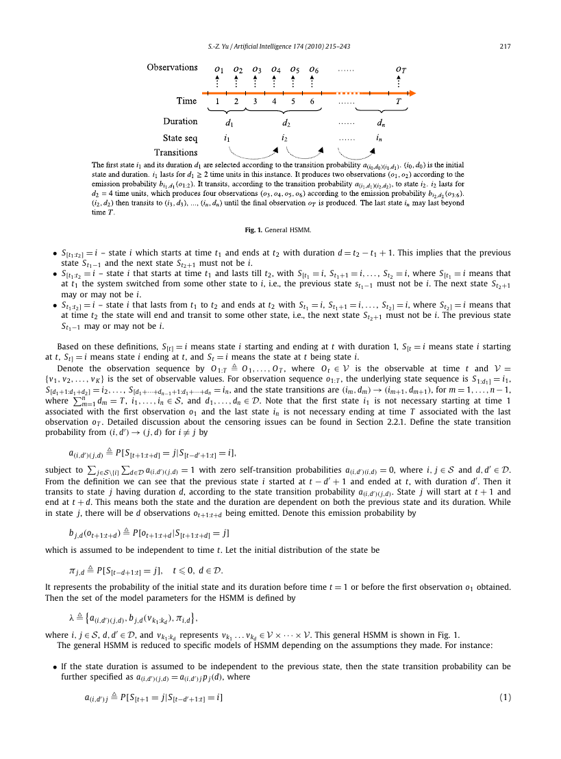
Fig. 1. General HSMM.
= i, where S[t1
= i, St1+1 = i, . . . , St2
= i – state i that starts at time t1 and lasts till t2, with S[t1
• S[t1:t2] = i – state i which starts at time t1 and ends at t2 with duration d = t2 − t1 + 1. This implies that the previous
state St1−1 and the next state St2+1 must not be i.
= i means that
• S[t1:t2
at t1 the system switched from some other state to i, i.e., the previous state st1−1 must not be i. The next state St2+1
may or may not be i.
= i, St1+1 = i, . . . , St2] = i, where St2] = i means that
• St1:t2] = i – state i that lasts from t1 to t2 and ends at t2 with St1
at time t2 the state will end and transit to some other state, i.e., the next state St2+1 must not be i. The previous state
St1−1 may or may not be i.
Based on these definitions, S[t] = i means state i starting and ending at t with duration 1, S[t = i means state i starting
at t, St] = i means state i ending at t, and St = i means the state at t being state i.
Denote the observation sequence by O 1:T O 1, . . . , O T , where O t ∈ V is the observable at time t and V =
{v1, v2, . . . , v K} is the set of observable values. For observation sequence o1:T , the underlying state sequence is S1:d1] = i1,
= in, and the state transitions are (im, dm) → (im+1, dm+1), for m = 1, . . . , n− 1,
S[d1+1:d1+d2] = i2, . . . , S[d1+···+dn−1+1:d1+···+dn
m=1 dm = T , i1, . . . , in ∈ S, and d1, . . . , dn ∈ D. Note that the first state i1 is not necessary starting at time 1
where
associated with the first observation o1 and the last state in is not necessary ending at time T associated with the last
observation oT . Detailed discussion about the censoring issues can be found in Section 2.2.1. Define the state transition
probability from (i, d
n
j∈S\{i}
)( j,d) P[S[t+1:t+d] = j|S[t−d+1:t] = i],
a(i,d
∈ D.
subject to
From the definition we can see that the previous state i started at t − d
. Then it
)( j,d). State j will start at t + 1 and
transits to state j having duration d, according to the state transition probability a(i,d
end at t + d. This means both the state and the duration are dependent on both the previous state and its duration. While
in state j, there will be d observations ot+1:t+d being emitted. Denote this emission probability by
)( j,d) = 1 with zero self-transition probabilities a(i,d
+ 1 and ended at t, with duration d
)(i,d) = 0, where i, j ∈ S and d, d
) → ( j, d) for i = j by
d∈D a(i,d
b j,d(ot+1:t+d) P[ot+1:t+d|S[t+1:t+d] = j]
which is assumed to be independent to time t. Let the initial distribution of the state be
π j,d P[S[t−d+1:t] = j],
t 0, d ∈ D.
It represents the probability of the initial state and its duration before time t = 1 or before the first observation o1 obtained.
Then the set of the model parameters for the HSMM is defined by
λ
a(i,d
where i, j ∈ S, d, d
)( j,d), b j,d(vk1:kd ), πi,d
∈ D, and vk1:kd represents vk1 . . . vkd
,
∈ V × ··· × V. This general HSMM is shown in Fig. 1.
The general HSMM is reduced to specific models of HSMM depending on the assumptions they made. For instance:
• If the state duration is assumed to be independent to the previous state, then the state transition probability can be
further specified as a(i,d
)( j,d) = a(i,d
) j p j(d), where
) j P[S[t+1 = j|S[t−d+1:t] = i]
a(i,d
(1)
�
218
S.-Z. Yu / Artificial Intelligence 174 (2010) 215–243
is the transition probability from state i that has stayed for duration d
to state j that will start at t + 1, and
p j(d) P[St+1:t+d] = j|S[t+1 = j]
(2)
is the probability of duration d that state j takes. This is the model proposed by Marhasev et al. [119].
• If a state transition is assumed to be independent to the duration of the previous state, then the state transition
probability becomes a(i,d
)( j,d) = ai( j,d), where
ai( j,d) P[S[t+1:t+d] = j|St] = i]
(3)
is the transition probability that state i ended at t and transits to state j having duration d. This is the residential time
HMM (see Section 3.3 for details). In this model, a state transition for i = j is (i, 1) → ( j, τ ) and a self-transition is
assumed to be (i, τ ) → (i, τ − 1) for τ > 1, where τ represents the residential time of the state.
• If a self-transition is allowed and is assumed to be independent to the previous state, then the state transition proba-
bility becomes
)( j,d) = a(i,d
) j
a(i,d
a jj(τ )
d−1
τ=1
1 − a jj(d)
,
where a jj(d) P[St+d+1 = j|S[t−d+1:t] = i, S[t+1:t+d = j] = P[St+d+1 = j|S[t+1:t+d = j] is the self-transition probability
when state j has stayed for d time units, and 1− a jj(d) = P[St+d] = j|S[t+1:t+d = j] is the probability state j ends with
duration d. This is the variable transition HMM (see Section 3.2 for details). In this model, a state transition is either
(i, d) → ( j, 1) for i = j or (i, d) → (i, d + 1) for a self-transition.
• If a transition to the current state is independent to the duration of the previous state and the duration is only condi-
)( j,d) = aij p j(d), where aij P[S[t+1 = j|St] = i] is the transition probability from
tioned on the current state, then a(i,d
state i to j, with the self-transition probability aii = 0. This is the explicit duration HMM (see Section 3.1 for details).
Besides, the state duration distributions, p j(d), can be parametric or non-parametric. The detailed discussion on various
duration distributions can be found in Section 4.1. Similarly, the observation distributions b j,d(vk1:kd ) can be parametric or
non-parametric, discrete or continuous, and dependent or independent on the state durations. It can also be a mixture of
distributions. The detailed discussion on various observation distributions can be found in Section 4.2.
2.2. Inference
In this subsection we discuss the issues related to inference, including the forward–backward algorithm, calculation of
probabilities and expectations, maximum a posteriori (MAP) estimate of states, maximum likelihood estimate (MLE) of state
sequence, and constrained estimate of states.
2.2.1. The forward–backward algorithm
We define the forward variables for HSMM by:
αt ( j, d) P[S[t−d+1:t] = j, o1:t|λ]
and the backward variables by
βt ( j, d) P[ot+1:T|S[t−d+1:t] = j, λ].
· a(i,d
αt ( j, d) =
αt−d
i, d
d∈D
for t > 0, d ∈ D, j ∈ S, and
d∈D
i∈S\{ j}
i∈S\{ j}
βt ( j, d) =
Similar to deriving the formulas for the HMM (see e.g., Rabiner [150], Ephraim and Merhav [57]), it is easy to obtain the
forward–backward algorithm for a general HSMM:
)( j,d) · b j,d(ot−d+1:t ),
i, d
,
(4)
(5)
a( j,d)(i,d
) · bi,d (ot+1:t+d ) · βt+d
for t < T .
The initial conditions generally can have two different assumptions:
• The general assumption: assumes that the first state begins at or before observation o1 and the last state ends at or after
observation oT . In this case, we can assume that the process starts at −∞ and terminates at +∞. The observations out
of the sampling period [1, T] can be any possible values, i.e., b j,d(·) = 1 for any j ∈ S, d ∈ D. Therefore, in the forward
�
S.-Z. Yu / Artificial Intelligence 174 (2010) 215–243
219
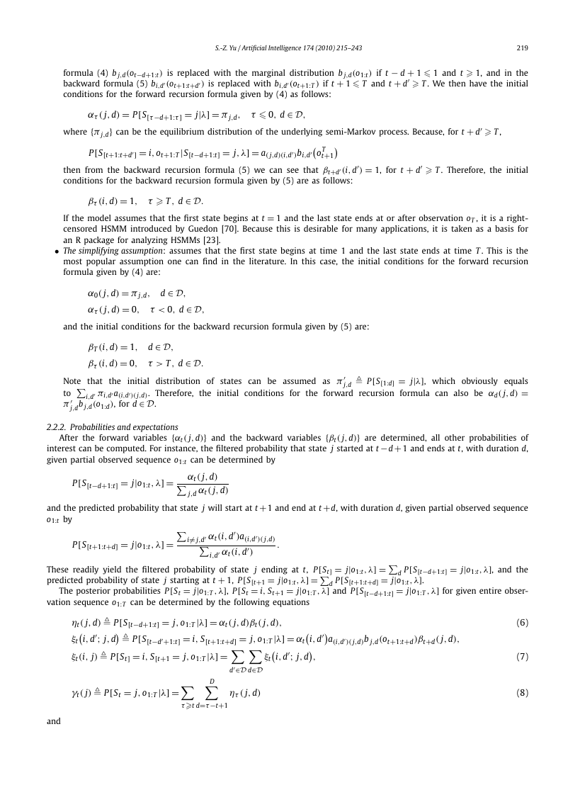
formula (4) b j,d(ot−d+1:t ) is replaced with the marginal distribution b j,d(o1:t ) if t − d + 1 1 and t 1, and in the
backward formula (5) bi,d (ot+1:t+d ) is replaced with bi,d (ot+1:T ) if t + 1 T and t + d
T . We then have the initial
conditions for the forward recursion formula given by (4) as follows:
ατ ( j, d) = P[S[τ−d+1:τ] = j|λ] = π j,d,
τ 0, d ∈ D,
where {π j,d} can be the equilibrium distribution of the underlying semi-Markov process. Because, for t + d
T ,
P[S[t+1:t+d] = i, ot+1:T|S[t−d+1:t] = j, λ] = a( j,d)(i,d
)bi,d
t+1
oT
then from the backward recursion formula (5) we can see that βt+d (i, d
conditions for the backward recursion formula given by (5) are as follows:
) = 1, for t + d
T . Therefore, the initial
βτ (i, d) = 1,
τ T , d ∈ D.
If the model assumes that the first state begins at t = 1 and the last state ends at or after observation oT , it is a right-
censored HSMM introduced by Guedon [70]. Because this is desirable for many applications, it is taken as a basis for
an R package for analyzing HSMMs [23].
• The simplifying assumption: assumes that the first state begins at time 1 and the last state ends at time T . This is the
most popular assumption one can find in the literature. In this case, the initial conditions for the forward recursion
formula given by (4) are:
α0( j, d) = π j,d,
ατ ( j, d) = 0,
d ∈ D,
τ < 0, d ∈ D,
and the initial conditions for the backward recursion formula given by (5) are:
βT (i, d) = 1,
βτ (i, d) = 0,
d ∈ D,
τ > T , d ∈ D.
Note that
to
j,db j,d(o1:d), for d ∈ D.
π
i,d πi,da(i,d
the initial distribution of states can be assumed as π
P[S[1:d] = j|λ], which obviously equals
)( j,d). Therefore, the initial conditions for the forward recursion formula can also be αd( j, d) =
j,d
2.2.2. Probabilities and expectations
After the forward variables {αt ( j, d)} and the backward variables {βt ( j, d)} are determined, all other probabilities of
interest can be computed. For instance, the filtered probability that state j started at t−d+ 1 and ends at t, with duration d,
given partial observed sequence o1:t can be determined by
P[S[t−d+1:t] = j|o1:t , λ] = αt ( j, d)
j,d αt ( j, d)
and the predicted probability that state j will start at t+1 and end at t+d, with duration d, given partial observed sequence
o1:t by
i= j,d αt (i, d
)a(i,d
i,d αt (i, d
)
)( j,d)
P[S[t+1:t+d] = j|o1:t , λ] =
These readily yield the filtered probability of state j ending at t, P[St] = j|o1:t , λ] =
predicted probability of state j starting at t + 1, P[S[t+1 = j|o1:t , λ] =
d P[S[t−d+1:t] = j|o1:t , λ], and the
The posterior probabilities P[St = j|o1:T , λ], P[St = i, St+1 = j|o1:T , λ] and P[S[t−d+1:t] = j|o1:T , λ] for given entire obser-
d P[S[t+1:t+d] = j|o1:t , λ].
.
vation sequence o1:T can be determined by the following equations
ξt
i, d
; j, d
P[S[t−d+1:t] = i, S[t+1:t+d] = j, o1:T|λ] = αt
; j, d
ηt ( j, d) P[S[t−d+1:t] = j, o1:T|λ] = αt ( j, d)βt ( j, d),
ξt (i, j) P[St] = i, S[t+1 = j, o1:T|λ] =
D
d=τ−t+1
γt ( j) P[St = j, o1:T|λ] =
d∈D
d∈D
ητ ( j, d)
τt
ξt
i, d
i, d
,
a(i,d
)( j,d)b j,d(ot+1:t+d)βt+d( j, d),
(6)
(7)
(8)
and
�
220
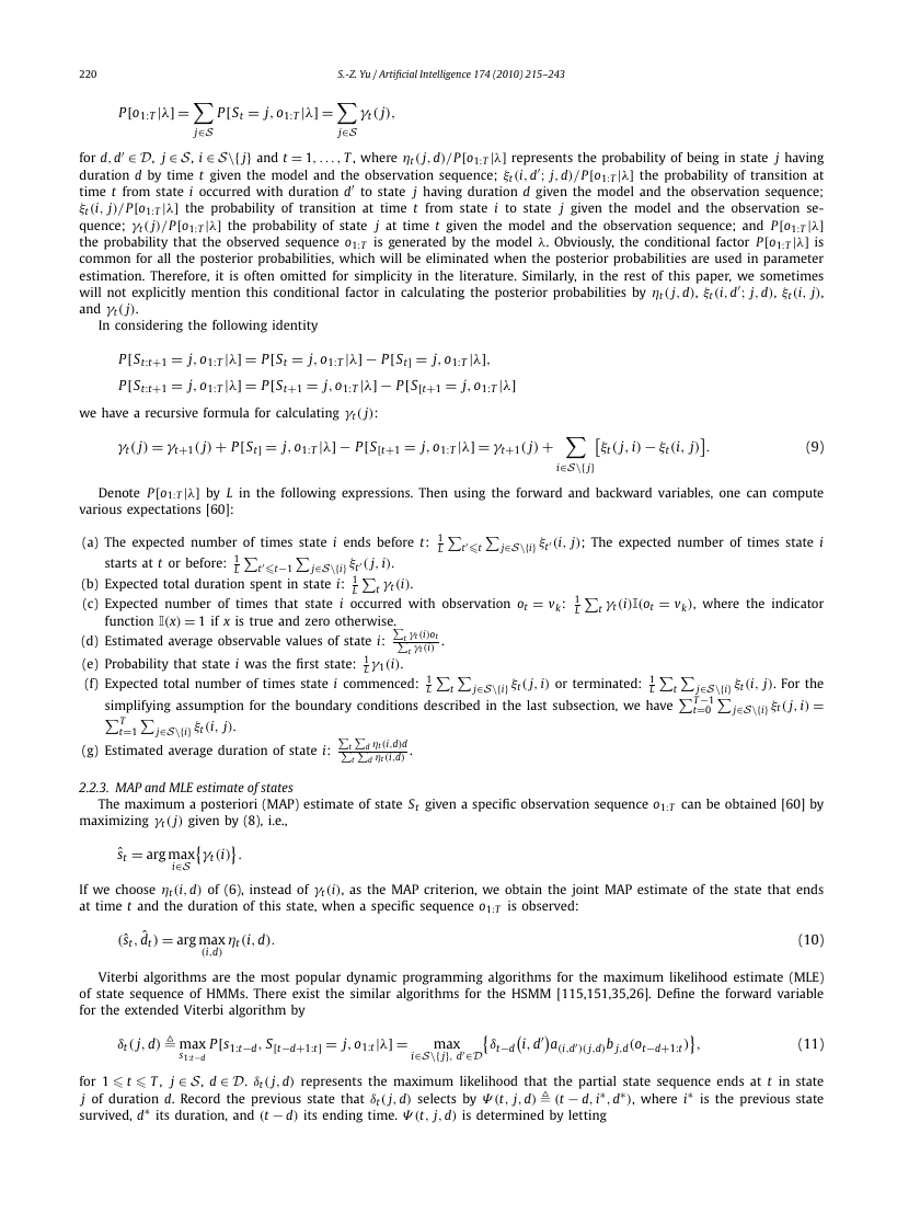
S.-Z. Yu / Artificial Intelligence 174 (2010) 215–243
j∈S
j∈S
γt ( j),
P[St = j, o1:T|λ] =
P[o1:T|λ] =
∈ D, j ∈ S, i ∈ S\{ j} and t = 1, . . . , T , where ηt ( j, d)/P[o1:T|λ] represents the probability of being in state j having
for d, d
; j, d)/P[o1:T|λ] the probability of transition at
duration d by time t given the model and the observation sequence; ξt (i, d
to state j having duration d given the model and the observation sequence;
time t from state i occurred with duration d
ξt (i, j)/P[o1:T|λ] the probability of transition at time t from state i to state j given the model and the observation se-
quence; γt ( j)/P[o1:T|λ] the probability of state j at time t given the model and the observation sequence; and P[o1:T|λ]
the probability that the observed sequence o1:T is generated by the model λ. Obviously, the conditional factor P[o1:T|λ] is
common for all the posterior probabilities, which will be eliminated when the posterior probabilities are used in parameter
estimation. Therefore, it is often omitted for simplicity in the literature. Similarly, in the rest of this paper, we sometimes
; j, d), ξt (i, j),
will not explicitly mention this conditional factor in calculating the posterior probabilities by ηt ( j, d), ξt (i, d
and γt ( j).
In considering the following identity
P[St:t+1 = j, o1:T|λ] = P[St = j, o1:T|λ] − P[St] = j, o1:T|λ],
P[St:t+1 = j, o1:T|λ] = P[St+1 = j, o1:T|λ] − P[S[t+1 = j, o1:T|λ]
we have a recursive formula for calculating γt ( j):
γt ( j) = γt+1( j) + P[St] = j, o1:T|λ] − P[S[t+1 = j, o1:T|λ] = γt+1( j) +
i∈S\{ j}
ξt ( j, i) − ξt (i, j)
.
(9)
Denote P[o1:T|λ] by L in the following expressions. Then using the forward and backward variables, one can compute
various expectations [60]:
tt−1
(b) Expected total duration spent in state i: 1
(c) Expected number of times that state i occurred with observation ot = vk: 1
L
starts at t or before: 1
L
(a) The expected number of times state i ends before t: 1
L
j∈S\{i} ξt ( j, i).
t γt (i).
function I(x) = 1 if x is true and zero otherwise.
(d) Estimated average observable values of state i:
(e) Probability that state i was the first state: 1
L γ1(i).
(f) Expected total number of times state i commenced: 1
L
t γt (i)ot
t γt (i)
.
j∈S\{i} ξt ( j, i) or terminated: 1
L
t
t
simplifying assumption for the boundary conditions described in the last subsection, we have
tt
j∈S\{i} ξt (i, j); The expected number of times state i
t γt (i)I(ot = vk), where the indicator
L
j∈S\{i} ξt (i, j). For the
T−1
j∈S\{i} ξt ( j, i) =
t=0
T
t=1
j∈S\{i} ξt (i, j).
(g) Estimated average duration of state i:
t
t
d ηt (i,d)d
d ηt (i,d)
.
The maximum a posteriori (MAP) estimate of state St given a specific observation sequence o1:T can be obtained [60] by
2.2.3. MAP and MLE estimate of states
maximizing γt ( j) given by (8), i.e.,
ˆst = arg max
i∈S
γt (i)
.
If we choose ηt (i, d) of (6), instead of γt (i), as the MAP criterion, we obtain the joint MAP estimate of the state that ends
at time t and the duration of this state, when a specific sequence o1:T is observed:
(ˆst ,
ˆdt ) = arg max
(i,d)
ηt (i, d).
(10)
Viterbi algorithms are the most popular dynamic programming algorithms for the maximum likelihood estimate (MLE)
of state sequence of HMMs. There exist the similar algorithms for the HSMM [115,151,35,26]. Define the forward variable
for the extended Viterbi algorithm by
P[s1:t−d, S[t−d+1:t] = j, o1:t|λ] =
δt ( j, d) max
(11)
s1:t−d
j ∈ S, d ∈ D. δt ( j, d) represents the maximum likelihood that the partial state sequence ends at t in state
∗ is the previous state
for 1 t T ,
j of duration d. Record the previous state that δt ( j, d) selects by Ψ (t, j, d) (t − d, i
∗
, d
∗ its duration, and (t − d) its ending time. Ψ (t, j, d) is determined by letting
survived, d
i∈S\{ j}, d∈D
), where i
a(i,d
δt−d
max
i, d
∗
)( j,d)b j,d(ot−d+1:t )
,
�
S.-Z. Yu / Artificial Intelligence 174 (2010) 215–243
i, d
δt−d
a(i,d
)( j,d)b j,d(ot−d+1:t )
.
221
Now the maximum likelihood state sequence can be determined by finding the last state that maximizes the likelihood. For
the general assumption of the boundary conditions on page 5, the last ML state is
or, for the simplifying assumption of the boundary conditions, t1 = T and
δt (i, d),
max
tT
i∈S
dt−T+1, d∈D
i∈S\{ j}, d∈D
∗
i
, d
t1, j
∗
1, d
j
. . .
t2, j
tn, j
∗
1
∗
1, d
∗ = arg max
= arg
= arg max
i∈S
d∈D
= Ψ
= Ψ
tn−1, j
∗
2, d
∗
∗
n, d
n
t1, j
∗
1
∗
2
δT (i, d).
,
∗
1, d
∗
1
,
∗
n−1, d
∗
n−1
Trace back the state sequence by letting
until the first state S1 is determined, where S1 = j
∗
n and ( j
∗
n, d
∗
n), . . . , ( j
∗
1, d
∗
1) is the maximum likelihood state sequence.
If the state duration density function is log-convex parametric, which is fulfilled by the commonly used parametric
functions, Bonafonte et al. [17] empirically showed that the computational complexity can be reduced to about 3.2 times of
the conventional HMM. If the model is a left–right HSMM or the particular state sequence, i1, . . . , in, is given, then only the
optimal segmentation of state durations needs to be determined. This is accomplished by simply rewriting (11) as [109,110]
δt (im, d) = max
d∈D
for 1 m n, 1 t T , d ∈ D.
δt−d
im−1, d
a(im−1,d
)(im,d)bim,d(ot−d+1:t )
,
2.2.4. Constrained estimate of states
As discussed in the previous subsections, the posterior probabilities P[St = j|o1:T , λ], P[St = i, St+1 = j|o1:T , λ] and
P[S[t−d+1:t] = j|o1:T , λ] for given entire observation sequence o1:T are determined by the forward–backward algorithm, and
are used for the computation of various expectations and the MAP estimation of states. These posterior probabilities can be
interpreted as the probabilities that the path taken (a random variable) passes through the constraint states for the given
observation sequence o1:T . For example, P[S[t−d+1:t] = j, o1:T|λ] = αt ( j, d)βt ( j, d) counts for all the paths that pass through
the constraint state j during the constraint period of t − d + 1 to t, where αt ( j, d) is given by (4) and βt ( j, d) by (5). This is
useful for the confidence calculation in the state estimation. The confidence can be simply defined as
max
j,d
αt ( j, d)βt ( j, d)
αt
j
,d
j
, d
j
, d
βt
,
where arg max j,d αt ( j, d)βt ( j, d) is used for the MAP estimate of the state as given by (10). Calculating the confidence over
every t, one can find out in practice when the errors are most likely to occur in the state estimation.
Now we compute the posterior probability P[st+1:t+k|o1:T , λ] corresponding to a segment of k observations. It is expected
useful in some applications. For example, this probability can be used to estimate the confidence of an individual field
of words for information extraction [41]. It can also be used for computing some expectations, which can be used for
estimating the states corresponding to the segment of k observations.
If one assumes that the first state of the subsequence st+1:t+k starts at t + 1 and the last state ends at t + k, i.e.,
st+1:t+k = ( j1, d1) . . . ( jn, dn), s.t. d1 + ··· + dn = k, it is easy to compute the posterior probability by
P[st+1:t+k, o1:T|λ] = αt+d1 ( j1, d1)
a( jm−1,dm−1)( jm,dm)b jm,dm (oτm−1+1:τm )
βt+k( jn, dn),
where τm = t + d1 + ··· + dm. When n = 1 the equation is reduced to (6). If we release the condition that the first state of
the subsequence starts at t + 1 or the one that the last state of the subsequence ends at t + k, the computation can be done
by allowing the first state duration d d1 and the last state duration d
dn.
A simple way for computing the posterior probability of a segment is modifying the forward–backward algorithm to con-
form the constraints. Similar to the constrained forward–backward algorithm for a CRF (conditional random field) proposed
by Culotta and McCallum [41], the forward–backward formulas given by (4) and (5) for the HSMM can be modified. Let
αt ( j, d) = 0 and βt ( j, d) = 0 when t + 1 t
t + k and j = st , where st ∈ st+1:t+k is a constraint that each path must pass
through and st+1:t+k is the constraint subpath. If we further constrain that the first state of the constraint subpath starts at
n
m=2
�
222
S.-Z. Yu / Artificial Intelligence 174 (2010) 215–243
− d + 1 < t + 1. Similarly, if we constrain that
t + 1, we must let αt ( j, d) = 0 and βt ( j, d) = 0 when t + 1 t
= P[st+1:t+k, o1:T|λ] =
− d+ 1 t + k and
the last state of the constraint subpath ends at t + k, we let αt ( j, d) = 0 and βt ( j, d) = 0 when t + 1 t
> t + k. Using this modified forward recursion, we obtain α
d∈D α
j∈S
T ( j, d) be
t
the constrained lattice, the set of all paths that conform to the constraints st+1:t+k. Then the posterior probability is yielded
/L, where L = P[o1:T|λ]. Obviously, the probabilities given by (6) to (8) can be computed using the modified forward
by L
recursion as well.
t + k and t
T ( j, d). Let L
2.3. Estimation
In the preceding problems, such as the forward–backward algorithm, MAP and ML estimation of states, we assumed that
the set of model parameters λ is given. If λ is unknown, we need to learn about λ from the observations o1:T : λ is initially
estimated and then re-estimated so that the likelihood function L(λ) = P[o1:T|λ] increases and converges to its maximum
value. If the system is slowly varying (i.e., non-stationary), the model parameters λ may need to be updated adaptively.
Such training and updating process is referred to as parameter re-estimation.
2.3.1. Parameter estimate of HSMM
For the parameter estimation/re-estimation problem, there is no known analytical method to find the λ that maximizes
the likelihood function. Thus, some iterative procedure must be employed.
t ξt (i, d
)( j,d) by
; j, d), and
The model parameters λ can be re-estimated using the expectations. For instance,
1) the initial distribution ˆπ j,d can be updated by ηt ( j, d)/
j,d ηt ( j, d) for t 0,
2) the transition probabilities ˆa(i,d
; j, d)/
j=i,d
3) the observation probabilities ˆb j,d(vk1:kd ) by
[ηt ( j, d) · I(ot+1:t+d = vk1:kd )]/
t ηt ( j, d), where I(ot+1:t+d = vk1:kd ) = 1
t ξt (i, d
if ot+1 = vk1 , . . . , ot+d = vkd and zero otherwise.
j=i
t ξt (i, j),
t ηt ( j, d)/
[γt ( j) · I(ot = vk)]/
d
Except these parameters for the general HSMM, parameters for other HSMMs can be estimated as well, such as
i) the transition probabilities ˆaij by
t ξt (i, j)/
ii) the duration probabilities ˆp j(d) of state j by
iii) the observation probabilities ˆb j(vk) by
iv) the initial distribution ˆπ j by γ0( j)/
t ηt ( j, d),
t γt ( j), and
ˆp j(d) = 1,
)( j,d) = 1,
ˆπ j,d = 1,
t
j γ0( j).
ˆa(i,d
j=i,d
d
j,d
t
Those probability mass function or probability density function satisfy:
ˆaij = 1,
j=i
The re-estimation procedure:
b j,d(vk1:kd ) = 1, and
b j(vk) = 1.
vk1 ,...,vkd
vk
a) Assume an initial model parameter set λ0;
b) For given model parameter set λk, use the forward–backward formulas (4) and (5) to compute the forward and
backward variables {αt ( j, d)} and {βt ( j, d)}. Then use the forward and backward variables to compute the related prob-
; j, d), ξt (i, j) and γt ( j) by (6) through (9). Finally re-estimate the model parameters to get
abilities ηt ( j, d), ξt (i, d
ˆλk+1;
c) Let λk+1 = ˆλk+1, k + +, and go back to step b);
d) Repeat b) and c) until the likelihood L(λk) = P[o1:T|λk] converges to a fixed point.
2.3.2. Order estimate of HSMM
In the re-estimation algorithms discussed above, the number of hidden states, M, the maximum length of state duration,
D, the number of observable values, K , and the length of the observation sequence, T , are usually assumed known in the
context of applications. However, the learning issues when the order of an HSMM is unknown is sometimes particularly
important in practice. A detailed discussion on the order estimate of HMMs can be found in Ephraim and Merhav [57,
Section VIII], and the issues of overfitting and model selection in Ghahramani [66, Section 7]. However, the order estimate
of HSMMs is somewhat different from that of HMMs, because HSMMs have variable durations. Therefore, for an HSMM we
must estimate both the number of states, M, and the maximum length of state durations, D.
In fact, some special HSMMs can be described by a dynamic Bayesian network (DBN) using a directed graphical model.
For simplicity, one usually assumes the observations are conditionally independent, i.e.,
b j,d(ot+1:t+d) = P[ot+1:t+d|S[t+1:t+d] = j] = t+d
(12)
where b j(vk) P[ot = vk|St = j]. To easily identify when a segment of states starts, one usually further assumes a state
transition is independent to the previous state duration. This is just the assumption made for the explicit duration HMM and
τ=t+1
b j(oτ ),
�





 2023年江西萍乡中考道德与法治真题及答案.doc
 2012年重庆南川中考生物真题及答案.doc
 2013年江西师范大学地理学综合及文艺理论基础考研真题.doc
 2020年四川甘孜小升初语文真题及答案I卷.doc
 2020年注册岩土工程师专业基础考试真题及答案.doc
 2023-2024学年福建省厦门市九年级上学期数学月考试题及答案.doc
 2021-2022学年辽宁省沈阳市大东区九年级上学期语文期末试题及答案.doc
 2022-2023学年北京东城区初三第一学期物理期末试卷及答案.doc
 2018上半年江西教师资格初中地理学科知识与教学能力真题及答案.doc
 2012年河北国家公务员申论考试真题及答案-省级.doc
 2020-2021学年江苏省扬州市江都区邵樊片九年级上学期数学第一次质量检测试题及答案.doc
 2022下半年黑龙江教师资格证中学综合素质真题及答案.doc