A survey on Semi-, Self- and Unsupervised Techniques in Image Classification
Similarities, Differences & Combinations
Lars Schmarje, Monty Santarossa,Simon-Martin Schr¨oder, Reinhard Koch
Multimedia Information Processing Group, Kiel University, Germany
{las,msa,sms,rk}@informatik.uni-kiel.de
0
2
0
2
b
e
F
0
2
]
V
C
.
s
c
[
1
v
1
2
7
8
0
.
2
0
0
2
:
v
i
X
r
a
Abstract
While deep learning strategies achieve outstanding
results in computer vision tasks, one issue remains.
The current strategies rely heavily on a huge amount
of labeled data. In many real-world problems it is not
feasible to create such an amount of labeled training
data. Therefore, researchers try to incorporate un-
labeled data into the training process to reach equal
results with fewer labels. Due to a lot of concurrent
research, it is difficult to keep track of recent develop-
ments. In this survey we provide an overview of often
used techniques and methods in image classification
with fewer labels. We compare 21 methods.
In our
analysis we identify three major trends. 1. State-of-
the-art methods are scaleable to real world applica-
tions based on their accuracy. 2. The degree of super-
vision which is needed to achieve comparable results
to the usage of all labels is decreasing. 3. All meth-
ods share common techniques while only few meth-
ods combine these techniques to achieve better perfor-
mance. Based on all of these three trends we discover
future research opportunities.
1. Introduction
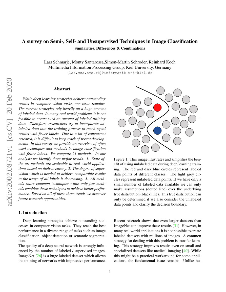
Figure 1: This image illustrates and simplifies the ben-
efit of using unlabeled data during deep learning train-
ing. The red and dark blue circles represent labeled
data points of different classes. The light grey cir-
cles represent unlabeled data points. If we have only a
small number of labeled data available we can only
make assumptions (dotted line) over the underlying
true distribution (black line). This true distribution can
only be determined if we also consider the unlabeled
data points and clarify the decision boundary.
Deep learning strategies achieve outstanding suc-
cesses in computer vision tasks. They reach the best
performance in a diverse range of tasks such as image
classification, object detection or semantic segmenta-
tion.
The quality of a deep neural network is strongly influ-
enced by the number of labeled / supervised images.
ImageNet [26] is a huge labeled dataset which allows
the training of networks with impressive performance.
Recent research shows that even larger datasets than
ImageNet can improve these results [31]. However, in
many real world applications it is not possible to create
labeled datasets with millions of images. A common
strategy for dealing with this problem is transfer learn-
ing. This strategy improves results even on small and
specialized datasets like medical imaging [40]. While
this might be a practical workaround for some appli-
cations, the fundamental issue remains: Unlike hu-
1
�
mans, supervised learning needs enormous amounts of
labeled data.
For a given problem we often have access to a large
dataset of unlabeled data. Xie et al. were among the
first to investigate unsupervised deep learning strate-
gies to leverage this data [45]. Since then, the usage of
unlabeled data has been researched in numerous ways
and has created research fields like semi-supervised,
self-supervised, weakly-supervised or metric learning
[23]. The idea that unifies these approaches is that us-
ing unlabeled data is beneficial during the training pro-
cess (see Figure 1 for an illustration). It either makes
the training with few labels more robust or in some
rare cases even surpasses the supervised cases [21].
Due to this benefit, many researchers and companies
work in the in the field of semi-, self- and unsupervised
learning. The main goal is to close the gap between
semi-supervised and supervised learning or even sur-
pass these results. Considering presented methods like
[49, 46] we believe that research is at the break point
of achieving this goal. Hence, there is a lot of research
ongoing in this field. This survey provides an overview
to keep track of the major and recent developments in
semi-, self- and unsupervised learning.
Most investigated research topics share a variety of
common ideas while differing in goal, application con-
texts and implementation details. This survey gives an
overview in this wide range of research topics. The fo-
cus of this survey is on describing the similarities and
differences between the methods. Moreover, we will
look at combinations of different techniques.
While we look at a broad range of learning strategies,
we compare these methods only based on the image
classification task. The addressed audience of this sur-
vey consists of deep learning researchers or interested
people with comparable preliminary knowledge who
want to keep track of recent developments in the field
of semi-, self- and unsupervised learning.
1.1. Related Work
In this subsection we give a quick overview about
previous works and reference topics we will not ad-
dress further in order to maintain the focus of this sur-
vey.
The research of semi- and unsupervised techniques in
computer vision has a long history. There has been a
variety of research and even surveys on this topic. Un-
supervised cluster algorithms were researched before
the breakthrough of deep learning and are still widely
used [30]. There are already extensive surveys that
describe unsupervised and semi-supervised strategies
without deep learning [47, 51]. We will focus only on
techniques including deep neural networks.
Many newer surveys focus only on self-, semi- or un-
supervised learning [33, 22, 44].
Min et al. wrote an overview about unsupervised deep
learning strategies [33]. They presented the beginning
in this field of research from a network architecture
perspective. The authors looked at a broad range of
architectures. We focus ourselves on only one archi-
tecture which Min et al. refer to as ”Clustering deep
neural network (CDNN)-based deep clustering” [33].
Even though the work was published in 2018, it al-
ready misses the recent development in deep learning
of the last years. We look at these more recent devel-
opments and show the connections to other research
fields that Min et al. didn’t include.
Van Engelen and Hoos give a broad overview about
general and recent semi-supervised methods [44].
While they cover some recent developments,
the
newest deep learning strategies are not covered. Fur-
thermore, the authors do not explicitly compare the
presented methods based on their structure or perfor-
mance. We provide such a comparison and also in-
clude self- and unsupervised methods.
Jing and Tian concentrated their survey on recent de-
velopments in self-supervised learning [22]. Like us
the authors provide an performance comparison and a
taxonomy. They do not compare the methods based on
their underlying techniques. Jing and Tian look at dif-
ferent tasks apart from classification but ignore semi-
and unsupervised methods.
Qi and Luo are one of the few who look at self-, semi-
and unsupervised learning in one survey [38]. How-
ever, they look at the different learning strategies sep-
arately and give comparison only inside the respective
learning strategy. We distinguish between these strate-
gies but we look also at the similarities between them.
We show that bridging these gaps leads to new in-
sights, improved performance and future research ap-
proaches.
Some surveys focus not on the general overviews
about semi-, self- and unsupervised learning but on
special details.
In their survey Cheplygina et al.
2
�
present a variety of methods in the context of med-
ical image analysis [6]. They include deep learning
and older machine learning approaches but look at dif-
ferent strategies from a medical perspective. Mey and
Loog focused on the underlying theoretical assump-
tions in semi-supervised learning [32]. We keep our
survey limited to general image classification tasks and
focus on their practical application.
Keeping the above mentioned limitations in mind the
topic of self-, semi- and unsupervised learning still in-
cludes a broad range of research fields. In this survey
we will focus on deep learning approaches for image
classification. We will investigate the different learn-
ing strategies with a spotlight on loss functions. There-
fore, topics like metric learning and general adversar-
ial networks will be excluded.
2. Underlying Concepts
In this section we summarize general ideas about
semi-, self- and unsupervised learning. We extend this
summarization by our own definition and interpreta-
tion of certain terms. The focus lies on distinguish-
ing the possible learning strategies and the most com-
mon methods to realize them. Throughout this sur-
vey we use the terms learning strategy, technique and
method in a specific meaning. The learning strategy
is the general type/approach of an algorithm. We call
each individual algorithm proposed in a paper method.
A method can be classified to a learning strategy and
consists out of techniques. Techniques are the parts or
ideas which make up the method/algorithm.
2.1. Learning strategies
Terms like supervised, semi-supervised and self-
supervised are often used in literature. A precise defi-
nition which clearly separates the terms is rarely given.
In most cases a rough general consensus about the
meaning is sufficient but we noticed a high variety of
definitions in borderline cases. For the comparison of
different methods we need a precise definition to dis-
tinguish between them. We will summarize the com-
mon consensus about the learning strategies and define
how we view certain borderline cases. In general, we
distinguish the methods based on the amount of used
labeled data and at which stage of the training process
supervision is introduced. Taken together, we call the
semi-, self- and unsupervised (learning) strategies re-
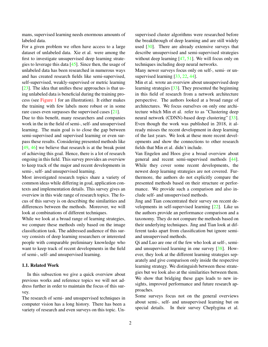
duced supervised (learning) strategies. Figure 2 illus-
trates the four presented deep learning strategies.
2.1.1 Supervised
Supervised learning is the most common strategy in
image classification with deep neural networks. We
have a set of images X and corresponding labels or
classes Z. Let C be the number of classes and f (x)
the output of a certain neural network for x ∈ X.
The goal is to minimize a loss function between the
outputs and labels. A common loss function to mea-
sure the difference between f (x) and the correspond-
ing label z is cross-entropy.
CE(f (x), z) =
C
Pf (x)(c)log(Pz(c))
= H(Pz)) + KL(Pz|Pf (x))
c=1
(1)
P is a probability distribution over all classes. H is
the entropy of a probability distribution and KL is
the Kullback-Leibler divergence. The distribution P
can be approximated with the output of neural net-
work f (x) or the given label z. It is important to note
that cross-entropy is the sum of entropy over z and a
Kullback-Leibler divergence between f (x) and z. In
general the entropy H(Pz) is zero due to one-hot en-
coded label z.
Transfer Learning
A limiting factor in supervised learning is the avail-
ability of labels. The creation of these labels can be ex-
pensive and therefore limits their number. One method
to overcome this limitation is to use transfer learning.
Transfer learning describes a two stage process of
training a neural network. The first stage is to train
with or without supervision on a large and generic
dataset like ImageNet [26]. The second stage is us-
ing the trained weights and fine-tune them on the tar-
get dataset. A great variety of papers have shown that
transfer learning can improve and stabilize the training
even on small domain-specific datasets [40].
2.1.2 Unsupervised
In unsupervised learning we only have images X and
no further labels. A variety of loss functions exist
3
�
(a) Supervised
(b) Semi-Supervised
(c) Unsupervised
(d) Self-Supervised
Figure 2: Illustrations of the four presented deep learning strategies - The red and dark blue circles represent
labeled data points of different classes. The light grey circles represent unlabeled data points. The black lines
define the underlying decision boundary between the classes. The striped circles represent datapoints which ignore
and use the label information at different stages of the training process.
in unsupervised learning [5, 21, 45].
In most cases
the problem is rephrased in such a way that all in-
puts for the loss can be generated, e.g. reconstruction
loss in auto encoders [45]. Despite this automation
or self-supervision we do call these methods unsuper-
vised. Please see below for our interpretation of self-
supervised learning.
2.1.3 Semi-Supervised
Semi-supervised learning is a mixture of unsupervised
and supervised learning. We have labels Z for a set
of images Xl like in supervised learning. The rest of
the images Xu have no corresponding label. Due to
this mixture, a semi-supervised loss can have a vari-
ety of shapes. A common way is to add a supervised
and an unsupervised loss. In contrast to other learning
strategies Xu and Xl are used in parallel.
2.1.4 Self-supervised
Self-supervised uses a pretext task to learn represen-
tations on unlabeled data. The pretext task is un-
supervised but the learned representations are often
not directly usable for image classification and have
to be fine-tuned. Therefore, self-supervised learning
can be interpreted either as an unsupervised, a semi-
supervised or a strategy of its own. We see self-
supervised learning as a special strategy. In the fol-
lowing, we will explain how we arrive at such a con-
clusion. The strategy cannot be call unsupervised if we
need to use any labels during the fine-tuning. There
is also a clear difference to semi-supervised methods.
The labels are not used simultaneously with unlabeled
data because the pretext task is unsupervised and only
the fine-tuning uses labels. For us this separation of
the usage of labeled data into two different subtasks
characterizes a strategy on its own.
2.2. Techniques
Different techniques can be used to train models in
reduced supervised cases. In this section we present a
selection of techniques that are used in multiple meth-
ods in the literature.
2.2.1 Consistency regularization
A major line of research uses consistency regulariza-
tion. In a semi-supervised learning process these reg-
ularizations are used as an additional loss to a super-
vised loss on the unsupervised part of the data. This
constraint leads to improved results due to the ability
of taking unlabeled data into account for defining the
decision boundaries [42, 28, 49]. Some self- or un-
supervised methods take this approach even further by
using only this consistency regularization for the train-
ing [21, 2].
Virtual Adversarial Training (VAT)
VAT [34] tries to make predictions invariant to small
transformations by minimizing the distance between
an image and a transformed version of the image. Miy-
ato et al. showed how a transformation can be chosen
and approximated in an adversarial way. This adver-
sarial transformation maximizes the distance between
4
�
an image and a transformed version of it over all pos-
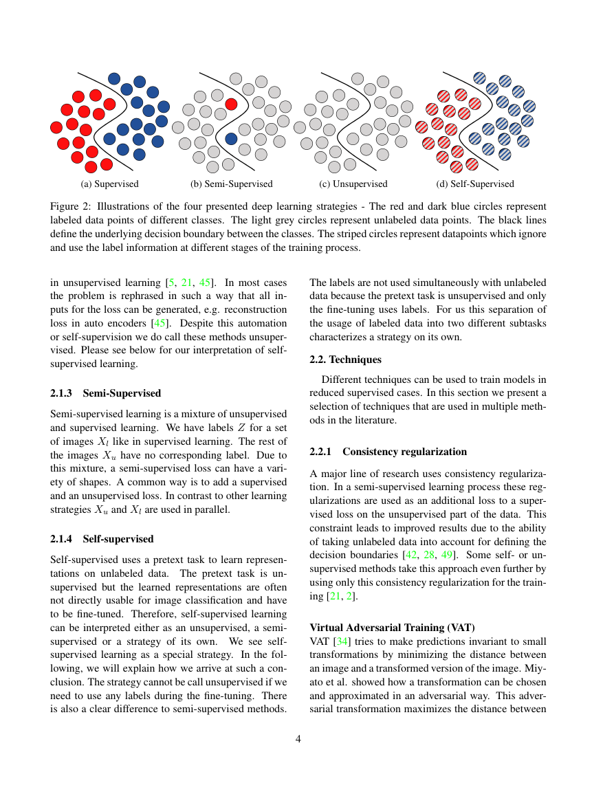
sible transformations. Figure 3 illustrates the concept
of VAT. The loss is defined as
V AT (f (x)) = D(Pf (x), Pf (x+radv))
radv = argmaxr;||r||≤�D(Pf (x), Pf (x+r))
(2)
In this equation x is an image out of the dataset X and
f (x) is the output for a given neural network. P is the
probability distribution over these outputs and D is a
non-negative function that measures the distance. Two
examples of used distance measures are cross-entropy
[34] and Kullback-Leiber divergence [49, 46].
Figure 3: Illustration of the VAT concept - The blue
and red circles represent two different classes. The line
is the decision boundary between these classes. The �
spheres around the circles define the area of possible
transformations. The arrows represent the adversarial
change r which push the decision boundary away from
any data point.
Mutual Information (MI)
MI is defined for two probability distributions as the
Kullback Leiber (KL) divergence between the joint
distribution and the marginal distributions [8]. This
measure is used as a loss function instead of CE in
several methods [19, 21, 2]. The benefits are described
below. For images x, y, certain neural network outputs
f (x), f (y) and the corresponding probability distribu-
tions Pf (x), Pf (y), we can maximize the mutual infor-
5
mation by minimizing the following:
−I(Pf (x), Pf (y)) = −KL(P(f (x),f (y))|Pf (x) ∗ Pf (y))
= −H(Pf (x)) + H(Pf (x)|Pf (y))
(3)
An alternative representation of mutual information is
the separation in entropy H(Pf (x)) and conditional en-
tropy H(Pf (x)|Pf (y)).
Ji et al. describe the benefits of using MI over CE in
unsupervised cases [21]. One major benefit is the in-
herent property to avoid degeneration due to the sepa-
ration in entropy and conditional entropy. MI balances
the effects of maximizing the entropy with a uniform
distribution for Pf (x) and minimizing the conditional
entropy by equalizing Pf (x) and Pf (y). Both cases are
undesirable for the output of a neural network.
Entropy Minimization (EntMin)
Grandvalet and Bengio proposed to sharpen the output
predictions in semi-supervised learning by minimizing
entropy [15]. They minimized the entropy H(Pf (x))
for all probability distributions Pf (x) based on a cer-
tain neural output f (x) for an image x. This minimiza-
tion only sharpens the predictions of a neural network
and cannot be used on it’s own.
Mean Squared Error (MSE)
A common distance measure between two neural net-
work outputs f (x), f (y) for images x, y is MSE. In-
stead of measuring the difference based on probability
theory it uses the euclidean distance of the output vec-
tors
M SE(f (x), f (y)) = ||f (x) − f (y)||2
2
(4)
The minimization of this measure can contract two
outputs to each other.
2.2.2 Overclustering
Normally, if we have k classes in a supervised case we
use also k clusters in an unsupervised case. Research
showed that it can be beneficial to use more clusters
than actual classes k exist [4, 21]. We call this idea
overclustering.
Overclustering can be beneficial in reduced supervised
�
cases due to the effect that neural networks can de-
cide ’on their own’ how to split the data. This sepa-
ration can be helpful in noisy data or with intermedi-
ate classes that were sorted into adjacent classes ran-
domly.
2.2.3 Pseudo-Labels
A simple approach for estimating labels of unknown
data are Pseudo-Labels [29]. Lee proposed to predict
classification for unseen data with a neural network
and use the predictions as labels. What sounds at first
like a self-fulfilling assumption works reasonably well
in real world image classification tasks. Several mod-
ern methods are based on the same core idea of creat-
ing labels by predicting them on their own [42, 3].
3. Methods
In the following, we give a short overview over all
methods in this survey in an alphabetical order and
separated according to their learning strategy. Due to
the fact that they may reference each other you may
have to jump to the corresponding entry if you would
like to know more. This list does not claim to be com-
plete. We included methods which were referenced of-
ten in related work, which are comparable to the other
methods and which are complementary to presented
methods.
3.1. Semi-Supervised
Fast-Stochastic Weight Averaging (fast-SWA)
In contrast to other semi-supervised methods Athi-
waratkun et al. do not change the loss but the opti-
mization algorithm [1]. They analysed the learning
process based on ideas and concepts of SWA [20],
π-model [28] and Mean Teacher [42]. Athiwaratkun
et al. show that averaging and cycling learning rates
are beneficial in semi-supervised learning by stabiliz-
ing the training. They call their improved version of
SWA fast-SWA due to a faster convergence and lower
performance variance [1]. The architecture and loss
is either copied from π-model [28] or Mean Teacher
[42].
Mean Teacher
With Mean Teacher Tarvainen & Valpola present a
student-teacher-approach for semi-supervised learning
[42]. They develop their approach based on the π-
model and Temporal Ensembling [28]. Therefore, they
also use MSE as a consistency loss between two pre-
dictions but create these predictions differently. They
argue that Temporal Ensembling incorporates new in-
formation too slowly into predictions. The reason for
this is that the exponential moving average (EMA) is
only updated once per epoch. Therefore, they propose
to use a teacher based on average weights of a stu-
dent in each update step. For their model Tarvainen
& Valpola show that the KL-divergence is an inferior
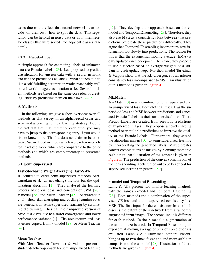
consistency loss in comparison to MSE. An illustration
of this method is given in Figure 4.
MixMatch
MixMatch [3] uses a combination of a supervised and
an unsupervised loss. Berthelot et al. use CE as the su-
pervised loss and MSE between predictions and gener-
ated Pseudo-Labels as their unsupervised loss. These
Pseudo-Labels are created from previous predictions
of augmented images. They propose a novel sharping
method over multiple predictions to improve the qual-
ity of the Pseudo-Labels. Furthermore, they extend
the algorithm mixup [50] to semi-supervised learning
by incorporating the generated labels. Mixup creates
convex combinations of images by blending them into
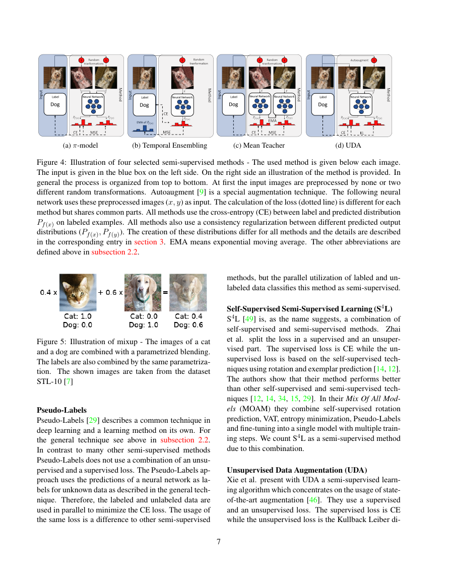
each other. An illustration of the concept is given in
Figure 5. The prediction of the convex combination of
the corresponding labels turned out to be beneficial for
supervised learning in general [50].
π-model and Temporal Ensembling
Laine & Aila present two similar learning methods
with the names π-model and Temporal Ensembling
[28]. Both methods use a combination of the super-
vised CE loss and the unsupervised consistency loss
MSE. The first input for the consistency loss in both
cases is the output of their network from a randomly
augmented input image. The second input is different
for each method. In the π-model a augmentation of
the same image is used. In Temporal Ensembling an
exponential moving average of previous predictions is
evaluated. Laine & Aila show that Temporal Ensem-
bling is up to two times faster and and more stable in
comparison to the π-model [28]. Illustrations of these
methods are given in Figure 4.
6
�
(a) π-model
(b) Temporal Ensembling
(c) Mean Teacher
(d) UDA
Figure 4: Illustration of four selected semi-supervised methods - The used method is given below each image.
The input is given in the blue box on the left side. On the right side an illustration of the method is provided. In
general the process is organized from top to bottom. At first the input images are preprocessed by none or two
different random transformations. Autoaugment [9] is a special augmentation technique. The following neural
network uses these preprocessed images (x, y) as input. The calculation of the loss (dotted line) is different for each
method but shares common parts. All methods use the cross-entropy (CE) between label and predicted distribution
Pf (x) on labeled examples. All methods also use a consistency regularization between different predicted output
distributions (Pf (x), Pf (y)). The creation of these distributions differ for all methods and the details are described
in the corresponding entry in section 3. EMA means exponential moving average. The other abbreviations are
defined above in subsection 2.2.
methods, but the parallel utilization of labled and un-
labeled data classifies this method as semi-supervised.
Self-Supervised Semi-Supervised Learning (S4L)
S4L [49] is, as the name suggests, a combination of
self-supervised and semi-supervised methods. Zhai
et al. split the loss in a supervised and an unsuper-
vised part. The supervised loss is CE while the un-
supervised loss is based on the self-supervised tech-
niques using rotation and exemplar prediction [14, 12].
The authors show that their method performs better
than other self-supervised and semi-supervised tech-
niques [12, 14, 34, 15, 29]. In their Mix Of All Mod-
els (MOAM) they combine self-supervised rotation
prediction, VAT, entropy minimization, Pseudo-Labels
and fine-tuning into a single model with multiple train-
ing steps. We count S4L as a semi-supervised method
due to this combination.
Unsupervised Data Augmentation (UDA)
Xie et al. present with UDA a semi-supervised learn-
ing algorithm which concentrates on the usage of state-
of-the-art augmentation [46]. They use a supervised
and an unsupervised loss. The supervised loss is CE
while the unsupervised loss is the Kullback Leiber di-
Figure 5: Illustration of mixup - The images of a cat
and a dog are combined with a parametrized blending.
The labels are also combined by the same parametriza-
tion. The shown images are taken from the dataset
STL-10 [7]
Pseudo-Labels
Pseudo-Labels [29] describes a common technique in
deep learning and a learning method on its own. For
the general technique see above in subsection 2.2.
In contrast to many other semi-supervised methods
Pseudo-Labels does not use a combination of an unsu-
pervised and a supervised loss. The Pseudo-Labels ap-
proach uses the predictions of a neural network as la-
bels for unknown data as described in the general tech-
nique. Therefore, the labeled and unlabeled data are
used in parallel to minimize the CE loss. The usage of
the same loss is a difference to other semi-supervised
7
�
(a) AMDIM
(b) CPC
(c) DeepCluster
(d) IIC
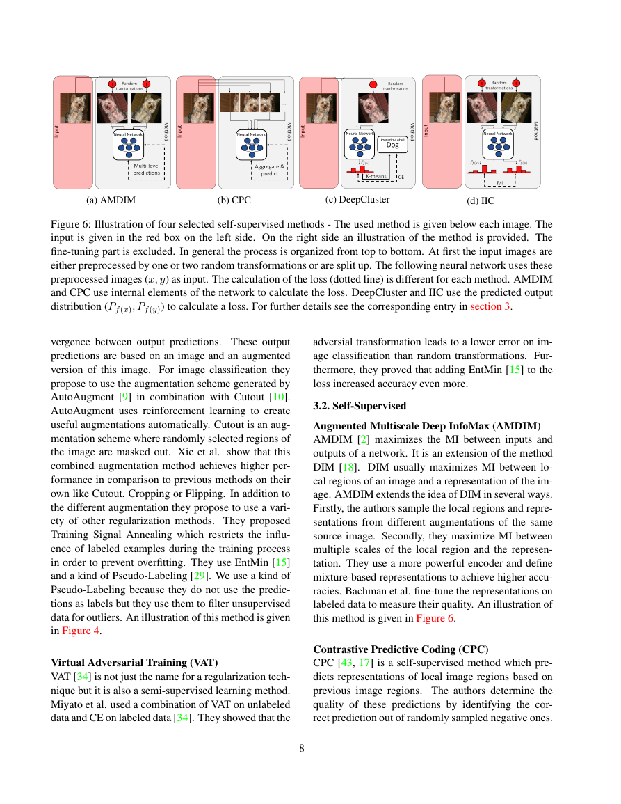
Figure 6: Illustration of four selected self-supervised methods - The used method is given below each image. The
input is given in the red box on the left side. On the right side an illustration of the method is provided. The
fine-tuning part is excluded. In general the process is organized from top to bottom. At first the input images are
either preprocessed by one or two random transformations or are split up. The following neural network uses these
preprocessed images (x, y) as input. The calculation of the loss (dotted line) is different for each method. AMDIM
and CPC use internal elements of the network to calculate the loss. DeepCluster and IIC use the predicted output
distribution (Pf (x), Pf (y)) to calculate a loss. For further details see the corresponding entry in section 3.
vergence between output predictions. These output
predictions are based on an image and an augmented
version of this image. For image classification they
propose to use the augmentation scheme generated by
AutoAugment [9] in combination with Cutout [10].
AutoAugment uses reinforcement learning to create
useful augmentations automatically. Cutout is an aug-
mentation scheme where randomly selected regions of
the image are masked out. Xie et al. show that this
combined augmentation method achieves higher per-
formance in comparison to previous methods on their
own like Cutout, Cropping or Flipping. In addition to
the different augmentation they propose to use a vari-
ety of other regularization methods. They proposed
Training Signal Annealing which restricts the influ-
ence of labeled examples during the training process
in order to prevent overfitting. They use EntMin [15]
and a kind of Pseudo-Labeling [29]. We use a kind of
Pseudo-Labeling because they do not use the predic-
tions as labels but they use them to filter unsupervised
data for outliers. An illustration of this method is given
in Figure 4.
Virtual Adversarial Training (VAT)
VAT [34] is not just the name for a regularization tech-
nique but it is also a semi-supervised learning method.
Miyato et al. used a combination of VAT on unlabeled
data and CE on labeled data [34]. They showed that the
adversial transformation leads to a lower error on im-
age classification than random transformations. Fur-
thermore, they proved that adding EntMin [15] to the
loss increased accuracy even more.
3.2. Self-Supervised
Augmented Multiscale Deep InfoMax (AMDIM)
AMDIM [2] maximizes the MI between inputs and
outputs of a network. It is an extension of the method
DIM [18]. DIM usually maximizes MI between lo-
cal regions of an image and a representation of the im-
age. AMDIM extends the idea of DIM in several ways.
Firstly, the authors sample the local regions and repre-
sentations from different augmentations of the same
source image. Secondly, they maximize MI between
multiple scales of the local region and the represen-
tation. They use a more powerful encoder and define
mixture-based representations to achieve higher accu-
racies. Bachman et al. fine-tune the representations on
labeled data to measure their quality. An illustration of
this method is given in Figure 6.
Contrastive Predictive Coding (CPC)
CPC [43, 17] is a self-supervised method which pre-
dicts representations of local image regions based on
previous image regions. The authors determine the
quality of these predictions by identifying the cor-
rect prediction out of randomly sampled negative ones.
8
�



 2023年江西萍乡中考道德与法治真题及答案.doc
 2012年重庆南川中考生物真题及答案.doc
 2013年江西师范大学地理学综合及文艺理论基础考研真题.doc
 2020年四川甘孜小升初语文真题及答案I卷.doc
 2020年注册岩土工程师专业基础考试真题及答案.doc
 2023-2024学年福建省厦门市九年级上学期数学月考试题及答案.doc
 2021-2022学年辽宁省沈阳市大东区九年级上学期语文期末试题及答案.doc
 2022-2023学年北京东城区初三第一学期物理期末试卷及答案.doc
 2018上半年江西教师资格初中地理学科知识与教学能力真题及答案.doc
 2012年河北国家公务员申论考试真题及答案-省级.doc
 2020-2021学年江苏省扬州市江都区邵樊片九年级上学期数学第一次质量检测试题及答案.doc
 2022下半年黑龙江教师资格证中学综合素质真题及答案.doc