stochastic calculus.pdf-资料库

invisiblepresley-3821128-4744302542860529660.pdf-第1页.png

第1页 / 共100页

invisiblepresley-3821128-4744302542860529660.pdf-第2页.png

第2页 / 共100页

invisiblepresley-3821128-4744302542860529660.pdf-第3页.png

第3页 / 共100页

invisiblepresley-3821128-4744302542860529660.pdf-第4页.png

第4页 / 共100页

invisiblepresley-3821128-4744302542860529660.pdf-第5页.png

第5页 / 共100页

invisiblepresley-3821128-4744302542860529660.pdf-第6页.png

第6页 / 共100页

invisiblepresley-3821128-4744302542860529660.pdf-第7页.png

第7页 / 共100页

invisiblepresley-3821128-4744302542860529660.pdf-第8页.png

第8页 / 共100页

StochasticCalculusAlan Bain

1. Introduction The following notes aim to provide a very informal introduction to Stochastic Calculus, and especially to the Itˆo integral and some of its applications. They owe a great deal to Dan Crisan’s Stochastic Calculus and Applications lectures of 1998; and also much to various books especially those of L. C. G. Rogers and D. Williams, and Dellacherie and Meyer’s multi volume series ‘Probabilities et Potentiel’. They have also beneﬁted from insights gained by attending lectures given by T. Kurtz. The present notes grew out of a set of typed notes which I produced when revising for the Cambridge, Part III course; combining the printed notes and my own handwritten notes into a consistent text. I’ve subsequently expanded them inserting some extra proofs from a great variety of sources. The notes principally concentrate on the parts of the course which I found hard; thus there is often little or no comment on more standard matters; as a secondary goal they aim to present the results in a form which can be readily extended Due to their evolution, they have taken a very informal style; in some ways I hope this may make them easier to read. The addition of coverage of discontinuous processes was motivated by my interest in the subject, and much insight gained from reading the excellent book of J. Jacod and A. N. Shiryaev. The goal of the notes in their current form is to present a fairly clear approach to the Itˆo integral with respect to continuous semimartingales but without any attempt at maximal detail. The various alternative approaches to this subject which can be found in books tend to divide into those presenting the integral directed entirely at Brownian Motion, and those who wish to prove results in complete generality for a semimartingale. Here at all points clarity has hopefully been the main goal here, rather than completeness; although secretly the approach aims to be readily extended to the discontinuous theory. I make no apology for proofs which spell out every minute detail, since on a ﬁrst look at the subject the purpose of some of the steps in a proof often seems elusive. I’d especially like to convince the reader that the Itˆo integral isn’t that much harder in concept than the Lebesgue Integral with which we are all familiar. The motivating principle is to try and explain every detail, no matter how trivial it may seem once the subject has been understood! Passages enclosed in boxes are intended to be viewed as digressions from the main text; usually describing an alternative approach, or giving an informal description of what is going on – feel free to skip these sections if you ﬁnd them unhelpful. In revising these notes I have resisted the temptation to alter the original structure of the development of the Itˆo integral (although I have corrected unintentional mistakes), since I suspect the more concise proofs which I would favour today would not be helpful on a ﬁrst approach to the subject. These notes contain errors with probability one. I always welcome people telling me about the errors because then I can ﬁx them! I can be readily contacted by email as alanb@chiark.greenend.org.uk. Also suggestions for improvements or other additions are welcome. Alan Bain [i]

2. Contents . . . . . . . . . . . . . . . . . . . . . . . . . . . . . . . . . . . . . . . . . . . . . . . . . . . . . . . . . . . . . . . 7. The Integral . 4.1. Stopping Times . . 1. Introduction . 2. Contents . . . 3. Stochastic Processes . 3.1. Probability Space . 3.2. Stochastic Process . . . . . . . . . . 5.1. Local Martingales . 5.2. Local Martingales which are not Martingales . . . . . . . . . . . . . . . . . . . . . 6. Total Variation and the Stieltjes Integral . . . . . . . . . . . . . . . . . . . . . . . . . . . . 10.1. The UCP topology 10.2. Approximation via Riemann Sums . . . 9. Semimartingales . 10. Relations to Sums 8. The Stochastic Integral 11. Itˆo’s Formula . . . . . . . . . . . . . . . . . . . . . . . . . . . . . . . . . . . . . . . . . . . . . . . . . . . . . . . . . . . . . . . . . . . . . . . . . . . . . . . . . . . . . . . . . . . . . . . . . . . . . . . . . . . . . . . . . . . . . . . . . . . . . . . . . . . . . . . . . . . . 5. Basics 4. Martingales 6.1. Why we need a Stochastic Integral . 6.2. Previsibility . 6.3. Lebesgue-Stieltjes Integral . . . . . . . . 7.1. Elementary Processes . 7.2. Strictly Simple and Simple Processes . . 8.1. Integral for H ∈ L and M ∈ M2 . . . 8.2. Quadratic Variation 8.3. Covariation . . . 8.4. Extension of the Integral to L2(M) 8.5. Localisation . 8.6. Some Important Results . . . . . . . . . . . . . . . . . . . . . . . . . . . . . . . . . . 12. L´evy Characterisation of Brownian Motion . . 13. Time Change of Brownian Motion . . . . . . . . . . . . . . . . . . . . . . . . . . . . . . . . . . . . . . . . . . . 15. Brownian Martingale Representation Theorem . . . 16. Stochastic Diﬀerential Equations . 17. Relations to Second Order PDEs . . . . . . 11.1. Applications of Itˆo’s Formula 11.2. Exponential Martingales . 13.1. Gaussian Martingales 14. Girsanov’s Theorem . 17.1. Inﬁnitesimal Generator . 17.2. The Dirichlet Problem . 14.1. Change of measure . . . . . . . . . . . . . . . . . . . . . . . . . . . . . . . . . . . . . . . . . . . . . . . . . . . . . . . . . . . . . . . . . . . . . . . . . . . . . . . . . . . . . . . . . . . . . . . . . . . . . . . . . . . . . . . . . . . . . . . . . . . . . . . . . . . . . . . . . . . . . . . . . . . . . . . . . . . . . . . . . . . . . . . . . . . . . . . . . . . . . . . . . . . . . . . . . . . . . . . . . . . . . . . . . . . . . . . . . . . . . . . . . . . . . . . . . . . . . . . . . . . . . . . . . . . . . . . . . . . . . . . . . . . . . . . . . . . . . . . . . . . . . . . . . . . . . . . . . . . . . . . . . . . . . . . . . . . . . . . . . . . . . . . . . . . . . . . . . . . . . . . . . . . . . . . . . . . . . . . . . . . . . . . . . . . . . . . . . . . . . . . . . . . . . . . . . . . . . . . . . . . . . . . . . . . . . . . . . . . . . . . . . . . . . . . . . . . . . . . . . i ii 1 1 1 4 4 8 8 9 11 11 12 13 15 15 15 17 17 19 22 23 26 27 29 31 31 32 35 40 41 46 48 49 51 51 53 56 61 61 62 [ii]

Contents iii 18. Stochastic Filtering . . . . . . . . . . . . . . . . . . . . . . . . . . . . . . . . . . . . . . . . . . . . . . . . . . . . . . . . . 17.3. The Cauchy Problem . . 17.4. Feynman-Ka˘c Representation . . . . . . . . . . . 18.1. Signal Process . 18.2. Observation Process . . 18.3. The Filtering Problem . . 18.4. Change of Measure . . 18.5. The Unnormalised Conditional Distribution . . 18.6. The Zakai Equation . 18.7. Kushner-Stratonowich Equation . . . . . . . . . . . . . . 21.1. Compensators . . 21.2. RCLL processes revisited . . . . . . . . . . . . . . . . . . . . . . . . . . . . . . . . . . . . . . . . . . . . . . . . . . . . . . . 19. Gronwall’s Inequality . . 20. Kalman Filter . . 20.1. Conditional Mean . . 20.2. Conditional Covariance . . . . . 21. Discontinuous Stochastic Calculus . . . 22. References . . . . . . . . . . . . . . . . . . . . . . . . . . . . . . . . . . . . . . . . . . . . . . . . . . . . . . . . . . . . . . . . . . . . . . . . . . . . . . . . . . . . . . . . . . . . . . . . . . . . . . . . . . . . . . . . . . . . . . . . . . . . . . . . . . . . . . . . . . . . . . . . . . . . . . . . . . . . . . . . . . . . . . . . . . . . . . . . . . . . . . . . . . . . . . . . . . . . . . . . . . . 64 66 69 69 70 70 70 76 78 86 87 89 89 90 92 92 94 96

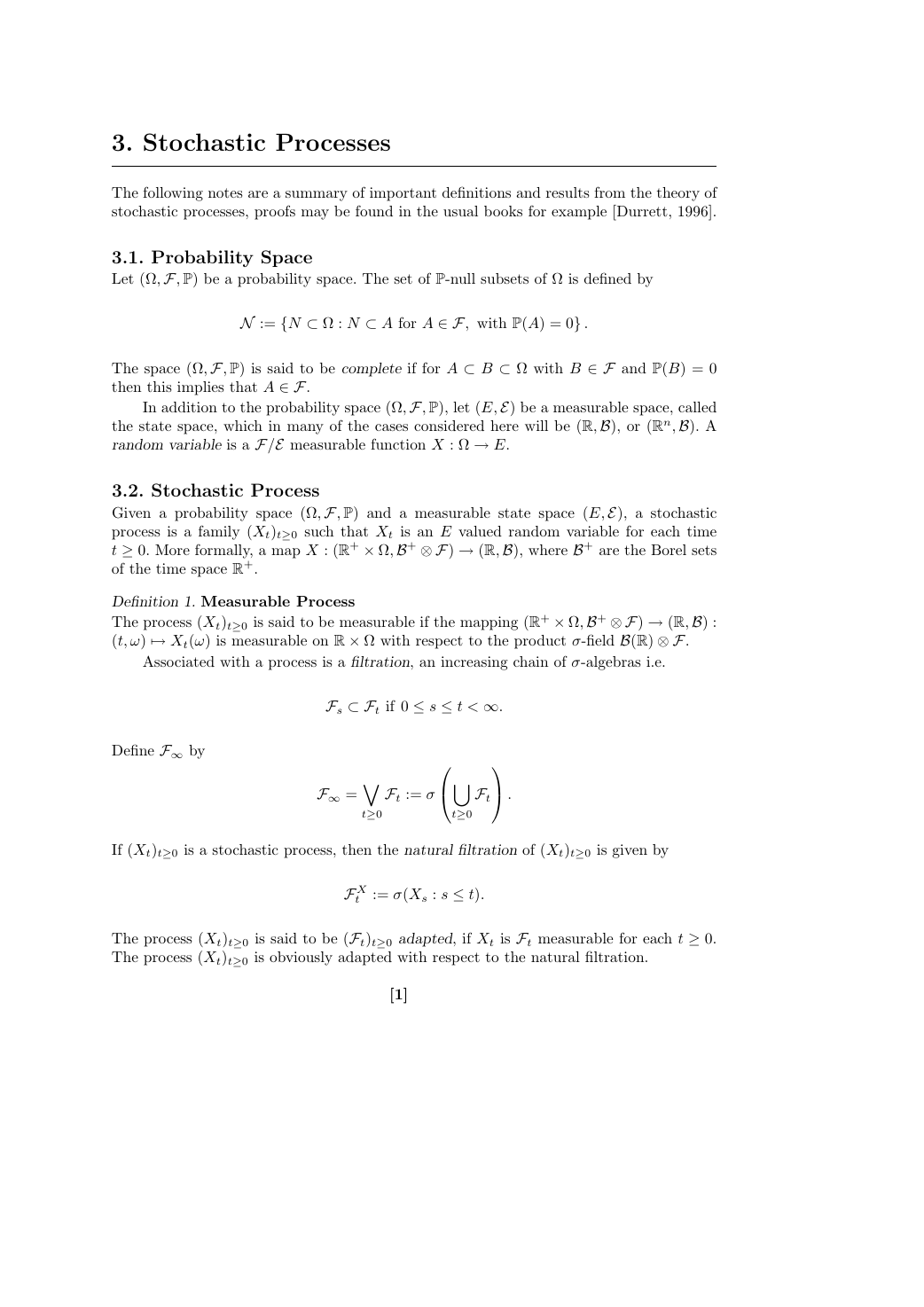
3. Stochastic Processes The following notes are a summary of important deﬁnitions and results from the theory of stochastic processes, proofs may be found in the usual books for example [Durrett, 1996]. 3.1. Probability Space Let (Ω,F, P) be a probability space. The set of P-null subsets of Ω is deﬁned by N := {N ⊂ Ω : N ⊂ A for A ∈ F, with P(A) = 0} . The space (Ω,F, P) is said to be complete if for A ⊂ B ⊂ Ω with B ∈ F and P(B) = 0 then this implies that A ∈ F. In addition to the probability space (Ω,F, P), let (E,E) be a measurable space, called the state space, which in many of the cases considered here will be (R,B), or (Rn,B). A random variable is a F/E measurable function X : Ω → E. 3.2. Stochastic Process Given a probability space (Ω,F, P) and a measurable state space (E,E), a stochastic process is a family (Xt)t≥0 such that Xt is an E valued random variable for each time t ≥ 0. More formally, a map X : (R+ × Ω,B+ ⊗ F) → (R,B), where B+ are the Borel sets of the time space R+. Deﬁnition 1. Measurable Process The process (Xt)t≥0 is said to be measurable if the mapping (R+ × Ω,B+ ⊗ F) → (R,B) : (t, ω) → Xt(ω) is measurable on R × Ω with respect to the product σ-ﬁeld B(R) ⊗ F. Associated with a process is a ﬁltration, an increasing chain of σ-algebras i.e. Deﬁne F∞ by Fs ⊂ Ft if 0 ≤ s ≤ t < ∞. F∞ = t≥0 Ft := σ  . Ft  t≥0 If (Xt)t≥0 is a stochastic process, then the natural ﬁltration of (Xt)t≥0 is given by F X t := σ(Xs : s ≤ t). The process (Xt)t≥0 is said to be (Ft)t≥0 adapted, if Xt is Ft measurable for each t ≥ 0. The process (Xt)t≥0 is obviously adapted with respect to the natural ﬁltration. [1]

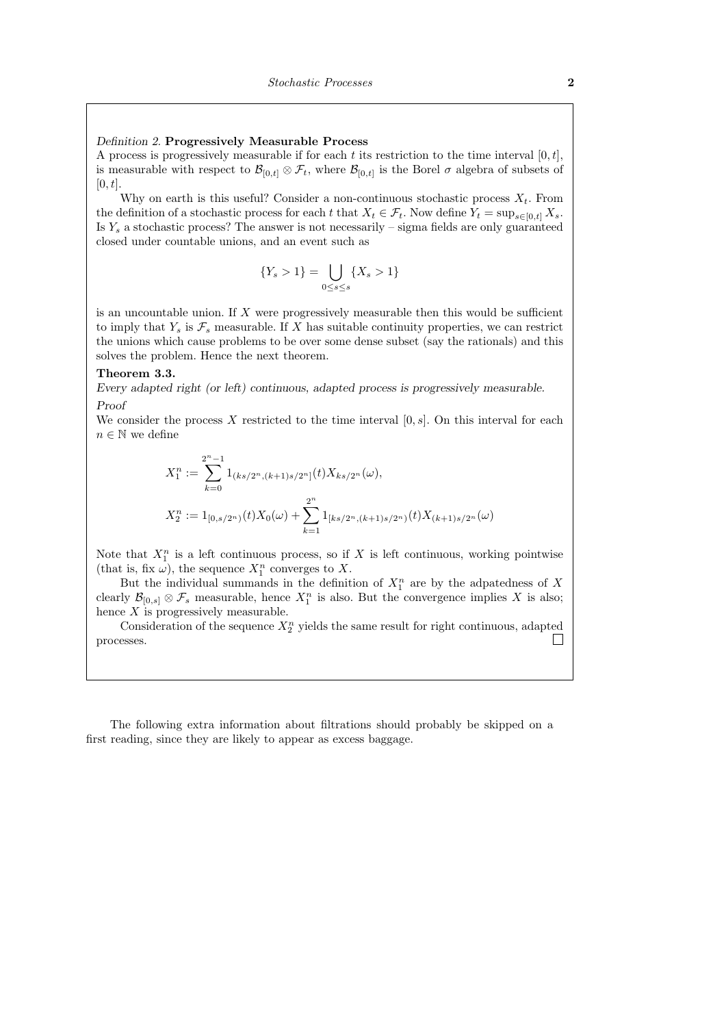
Stochastic Processes 2 Deﬁnition 2. Progressively Measurable Process A process is progressively measurable if for each t its restriction to the time interval [0, t], is measurable with respect to B[0,t] ⊗ Ft, where B[0,t] is the Borel σ algebra of subsets of [0, t]. Why on earth is this useful? Consider a non-continuous stochastic process Xt. From the deﬁnition of a stochastic process for each t that Xt ∈ Ft. Now deﬁne Yt = sups∈[0,t] Xs. Is Ys a stochastic process? The answer is not necessarily – sigma ﬁelds are only guaranteed closed under countable unions, and an event such as {Ys > 1} = 0≤s≤s {Xs > 1} is an uncountable union. If X were progressively measurable then this would be suﬃcient to imply that Ys is Fs measurable. If X has suitable continuity properties, we can restrict the unions which cause problems to be over some dense subset (say the rationals) and this solves the problem. Hence the next theorem. Theorem 3.3. Every adapted right (or left) continuous, adapted process is progressively measurable. Proof We consider the process X restricted to the time interval [0, s]. On this interval for each n ∈ N we deﬁne 2n−1 X n 1 := 1(ks/2n,(k+1)s/2n](t)Xks/2n(ω), k=0 X n 2 := 1[0,s/2n)(t)X0(ω) + 2n k=1 1[ks/2n,(k+1)s/2n)(t)X(k+1)s/2n(ω) 1 is a left continuous process, so if X is left continuous, working pointwise But the individual summands in the deﬁnition of X n 1 are by the adpatedness of X 1 is also. But the convergence implies X is also; Note that X n (that is, ﬁx ω), the sequence X n clearly B[0,s] ⊗ Fs measurable, hence X n hence X is progressively measurable. Consideration of the sequence X n 1 converges to X. processes. 2 yields the same result for right continuous, adapted The following extra information about ﬁltrations should probably be skipped on a ﬁrst reading, since they are likely to appear as excess baggage.

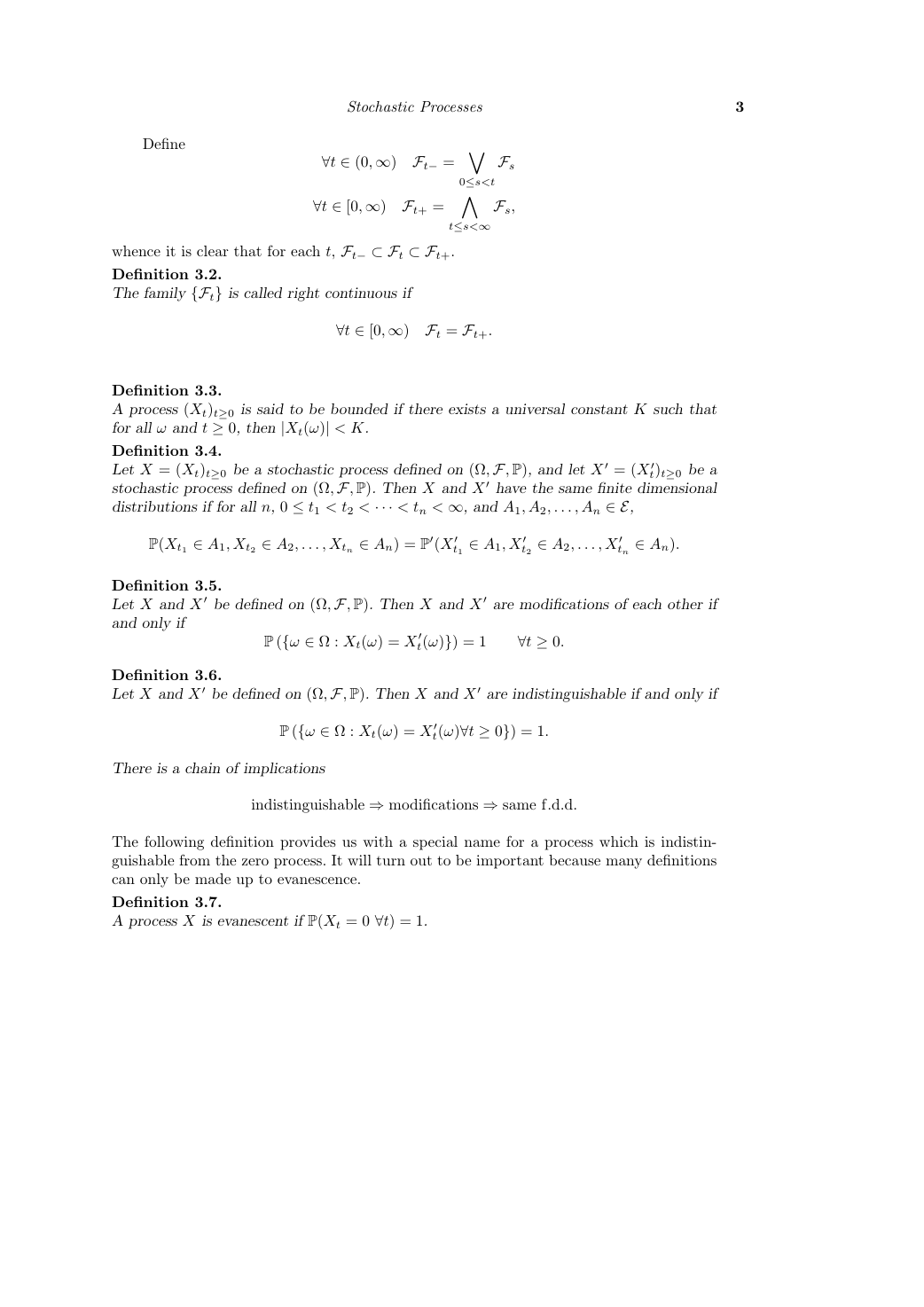
Deﬁne Stochastic Processes ∀t ∈ (0,∞) Ft− = ∀t ∈ [0,∞) Ft+ = 0≤s

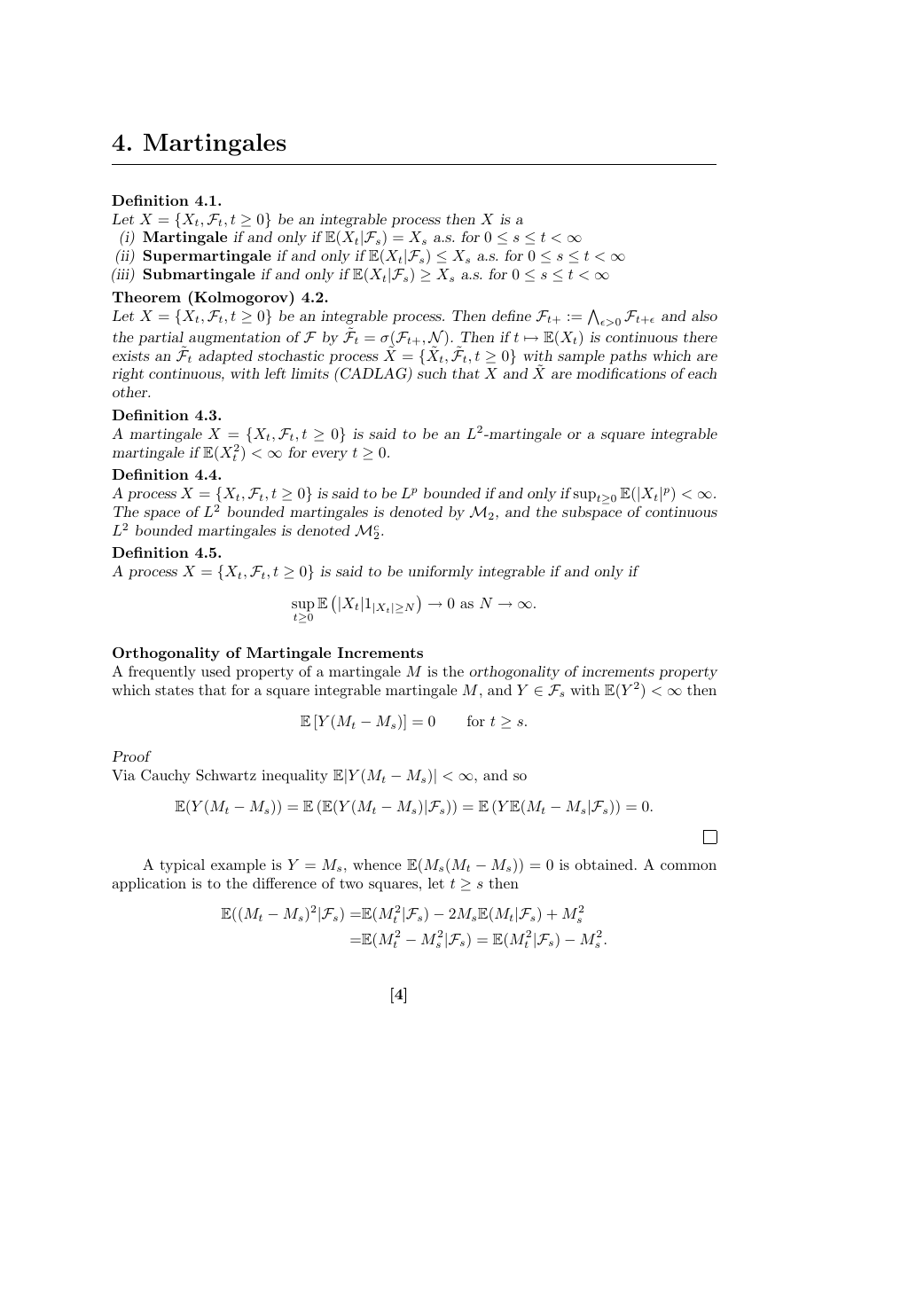
4. Martingales Let X = {Xt,Ft, t ≥ 0} be an integrable process. Then deﬁne Ft+ := Deﬁnition 4.1. Let X = {Xt,Ft, t ≥ 0} be an integrable process then X is a (i) Martingale if and only if E(Xt|Fs) = Xs a.s. for 0 ≤ s ≤ t < ∞ (ii) Supermartingale if and only if E(Xt|Fs) ≤ Xs a.s. for 0 ≤ s ≤ t < ∞ (iii) Submartingale if and only if E(Xt|Fs) ≥ Xs a.s. for 0 ≤ s ≤ t < ∞ Theorem (Kolmogorov) 4.2. >0 Ft+ and also the partial augmentation of F by ˜Ft = σ(Ft+,N ). Then if t → E(Xt) is continuous there exists an ˜Ft adapted stochastic process ˜X = { ˜Xt, ˜Ft, t ≥ 0} with sample paths which are right continuous, with left limits (CADLAG) such that X and ˜X are modiﬁcations of each other. Deﬁnition 4.3. A martingale X = {Xt,Ft, t ≥ 0} is said to be an L2-martingale or a square integrable martingale if E(X 2 Deﬁnition 4.4. E(|Xt|p) < ∞. A process X = {Xt,Ft, t ≥ 0} is said to be Lp bounded if and only if supt≥0 The space of L2 bounded martingales is denoted by M2, and the subspace of continuous L2 bounded martingales is denoted Mc 2. Deﬁnition 4.5. A process X = {Xt,Ft, t ≥ 0} is said to be uniformly integrable if and only if t ) < ∞ for every t ≥ 0. E|Xt|1|Xt|≥N → 0 as N → ∞. sup t≥0 Orthogonality of Martingale Increments A frequently used property of a martingale M is the orthogonality of increments property which states that for a square integrable martingale M, and Y ∈ Fs with E(Y 2) < ∞ then E [Y (Mt − Ms)] = 0 for t ≥ s. Proof Via Cauchy Schwartz inequality E|Y (Mt − Ms)| < ∞, and so E(Y (Mt − Ms)) = E (E(Y (Mt − Ms)|Fs)) = E (Y E(Mt − Ms|Fs)) = 0. A typical example is Y = Ms, whence E(Ms(Mt − Ms)) = 0 is obtained. A common application is to the diﬀerence of two squares, let t ≥ s then E((Mt − Ms)2|Fs) =E(M 2 =E(M 2 t |Fs) − 2MsE(Mt|Fs) + M 2 t − M 2 s |Fs) = E(M 2 t |Fs) − M 2 s . s [4]

资料库

stochastic calculus.pdf

相关推荐

课程资源

热门标签

最新资料