Bucknell University
Using ODE45
MATLAB Help
MATLAB's standard solver for ordinary differential equations (ODEs) is the function ode45. This
function implements a Runge-Kutta method with a variable time step for efficient computation.
ode45 id designed to handle the following general problem
y
d
dt
=
f
y
( , )
t
y
(
to
)
=
y
o
[1]
where t is the independent variable (time, position, volume) and y is a vector of dependent variables
(temperature, position, concentrations) to be found. The mathematical problem is specified when
the vector of functions on the right-hand side of Eq. [1], f
yo at time to, are specified.
, is set and the initial conditions, y =
y( , )
t
The notes here apply to versions of MATLAB above 5.0 and cover the basics of using the function
ode45. For more information on this and other ODE solvers in MATLAB, see the on-line help.
Contents:
Syntax for ode45 ....................................................................................................................... 2
Integrating a single, first-order equation...................................................................................... 3
Getting the solution at particular values of the independent variable........................................... 4
Integrating a set of coupled first-order equations......................................................................... 4
Integrating a second-order initial-value problem (IVP)................................................................ 7
Integrating an Nth-order initial-value problem............................................................................ 8
Changing model parameters........................................................................................................ 9
Integrating a second-order boundary-value problem (BVP)........................................................ 11
Setting options in ode45 .......................................................................................................... 12
Going beyond ode45................................................................................................................. 13
ENGR210
Using ODE45
1
�
Syntax for ode45
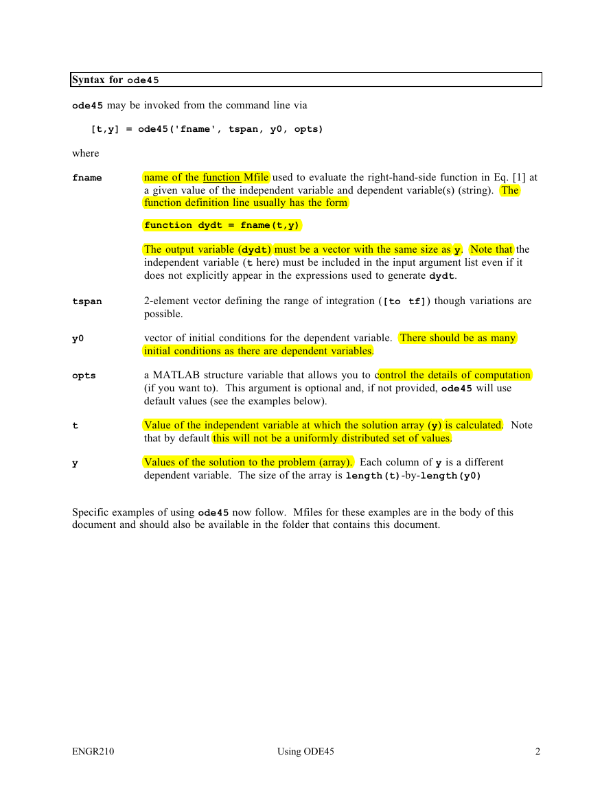
ode45 may be invoked from the command line via
[t,y] = ode45('fname', tspan, y0, opts)
where
fname
tspan
y0
opts
t
y
name of the function Mfile used to evaluate the right-hand-side function in Eq. [1] at
a given value of the independent variable and dependent variable(s) (string). The
function definition line usually has the form
function dydt = fname(t,y)
The output variable (dydt) must be a vector with the same size as y. Note that the
independent variable (t here) must be included in the input argument list even if it
does not explicitly appear in the expressions used to generate dydt.
2-element vector defining the range of integration ([to tf]) though variations are
possible.
vector of initial conditions for the dependent variable. There should be as many
initial conditions as there are dependent variables.
a MATLAB structure variable that allows you to control the details of computation
(if you want to). This argument is optional and, if not provided, ode45 will use
default values (see the examples below).
Value of the independent variable at which the solution array (y) is calculated. Note
that by default this will not be a uniformly distributed set of values.
Values of the solution to the problem (array). Each column of y is a different
dependent variable. The size of the array is length(t)-by-length(y0)
Specific examples of using ode45 now follow. Mfiles for these examples are in the body of this
document and should also be available in the folder that contains this document.
ENGR210
Using ODE45
2
�
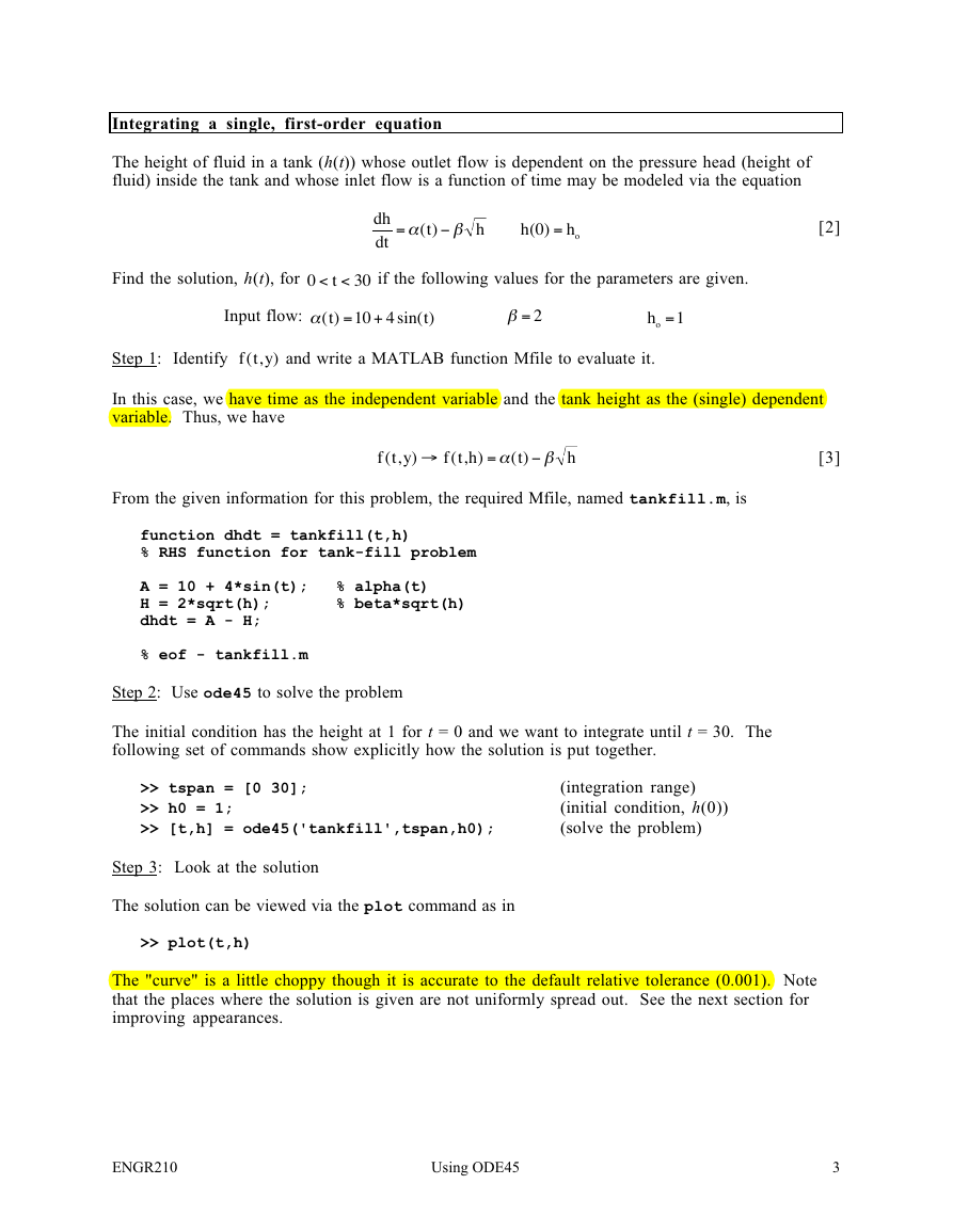
Integrating a single, first-order equation
The height of fluid in a tank (h(t)) whose outlet flow is dependent on the pressure head (height of
fluid) inside the tank and whose inlet flow is a function of time may be modeled via the equation
=
dh
dt
α β( )
−
t
h
h
( )0
=
ho
[2]
Find the solution, h(t), for 0
< > tspan = [0 30];
>> h0 = 1;
>> [t,h] = ode45('tankfill',tspan,h0);
(integration range)
(initial condition, h(0))
(solve the problem)
Step 3: Look at the solution
The solution can be viewed via the plot command as in
>> plot(t,h)
The "curve" is a little choppy though it is accurate to the default relative tolerance (0.001). Note
that the places where the solution is given are not uniformly spread out. See the next section for
improving appearances.
ENGR210
Using ODE45
3
�
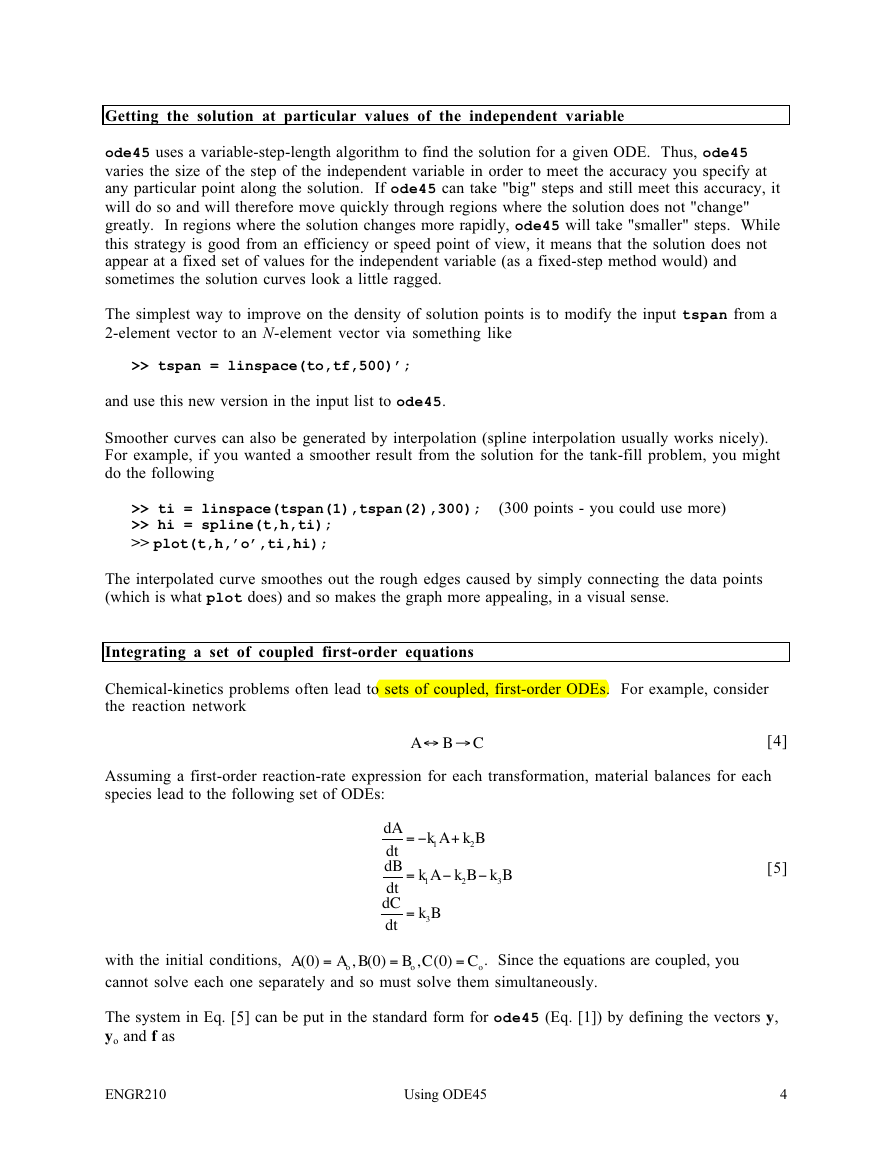
Getting the solution at particular values of the independent variable
ode45 uses a variable-step-length algorithm to find the solution for a given ODE. Thus, ode45
varies the size of the step of the independent variable in order to meet the accuracy you specify at
any particular point along the solution. If ode45 can take "big" steps and still meet this accuracy, it
will do so and will therefore move quickly through regions where the solution does not "change"
greatly. In regions where the solution changes more rapidly, ode45 will take "smaller" steps. While
this strategy is good from an efficiency or speed point of view, it means that the solution does not
appear at a fixed set of values for the independent variable (as a fixed-step method would) and
sometimes the solution curves look a little ragged.
The simplest way to improve on the density of solution points is to modify the input tspan from a
2-element vector to an N-element vector via something like
>> tspan = linspace(to,tf,500)’;
and use this new version in the input list to ode45.
Smoother curves can also be generated by interpolation (spline interpolation usually works nicely).
For example, if you wanted a smoother result from the solution for the tank-fill problem, you might
do the following
>> ti = linspace(tspan(1),tspan(2),300); (300 points - you could use more)
>> hi = spline(t,h,ti);
>> plot(t,h,’o’,ti,hi);
The interpolated curve smoothes out the rough edges caused by simply connecting the data points
(which is what plot does) and so makes the graph more appealing, in a visual sense.
Integrating a set of coupled first-order equations
Chemical-kinetics problems often lead to sets of coupled, first-order ODEs. For example, consider
the reaction network
↔ →
B C
A
[4]
Assuming a first-order reaction-rate expression for each transformation, material balances for each
species lead to the following set of ODEs:
dA
dt
dB
dt
dC
dt
= −
+
k A k B
1
2
=
=
−
k A k B k B
1
2
3
−
k B
3
[5]
with the initial conditions, A
cannot solve each one separately and so must solve them simultaneously.
B C
o
( )
0
A B
,
( )
0
( )
0
,
o
. Since the equations are coupled, you
=
C
o
=
=
The system in Eq. [5] can be put in the standard form for ode45 (Eq. [1]) by defining the vectors y,
yo and f as
ENGR210
Using ODE45
4
�
=
y
A
B
C
y
( )
0
=
y
o
=
A
o
B
o
C
o
f
y
( , )
t
=
−
k y
1 1
+
k y
k y
2
2
1 1
+
−
(
)
k y
k
3
2
k y
3
2
2
[6]
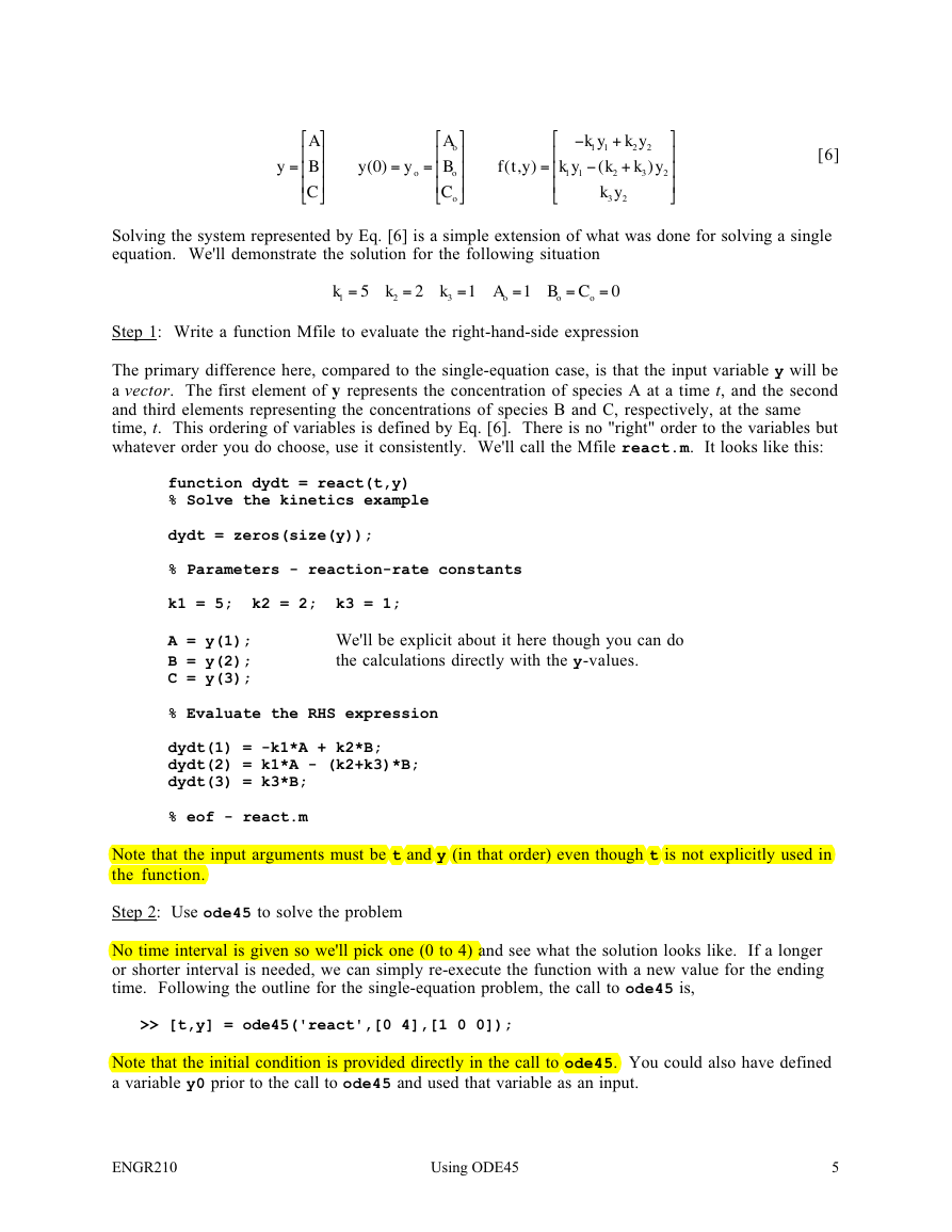
Solving the system represented by Eq. [6] is a simple extension of what was done for solving a single
equation. We'll demonstrate the solution for the following situation
=
5
k
1
=
2
k
2
=
1
k
3
=
1
A
o
=
B C
o
o
=
0
Step 1: Write a function Mfile to evaluate the right-hand-side expression
The primary difference here, compared to the single-equation case, is that the input variable y will be
a vector. The first element of y represents the concentration of species A at a time t, and the second
and third elements representing the concentrations of species B and C, respectively, at the same
time, t. This ordering of variables is defined by Eq. [6]. There is no "right" order to the variables but
whatever order you do choose, use it consistently. We'll call the Mfile react.m. It looks like this:
function dydt = react(t,y)
% Solve the kinetics example
dydt = zeros(size(y));
% Parameters - reaction-rate constants
k1 = 5; k2 = 2; k3 = 1;
A = y(1);
B = y(2);
C = y(3);
We'll be explicit about it here though you can do
the calculations directly with the y-values.
% Evaluate the RHS expression
dydt(1) = -k1*A + k2*B;
dydt(2) = k1*A - (k2+k3)*B;
dydt(3) = k3*B;
% eof - react.m
Note that the input arguments must be t and y (in that order) even though t is not explicitly used in
the function.
Step 2: Use ode45 to solve the problem
No time interval is given so we'll pick one (0 to 4) and see what the solution looks like. If a longer
or shorter interval is needed, we can simply re-execute the function with a new value for the ending
time. Following the outline for the single-equation problem, the call to ode45 is,
>> [t,y] = ode45('react',[0 4],[1 0 0]);
Note that the initial condition is provided directly in the call to ode45. You could also have defined
a variable y0 prior to the call to ode45 and used that variable as an input.
ENGR210
Using ODE45
5
�
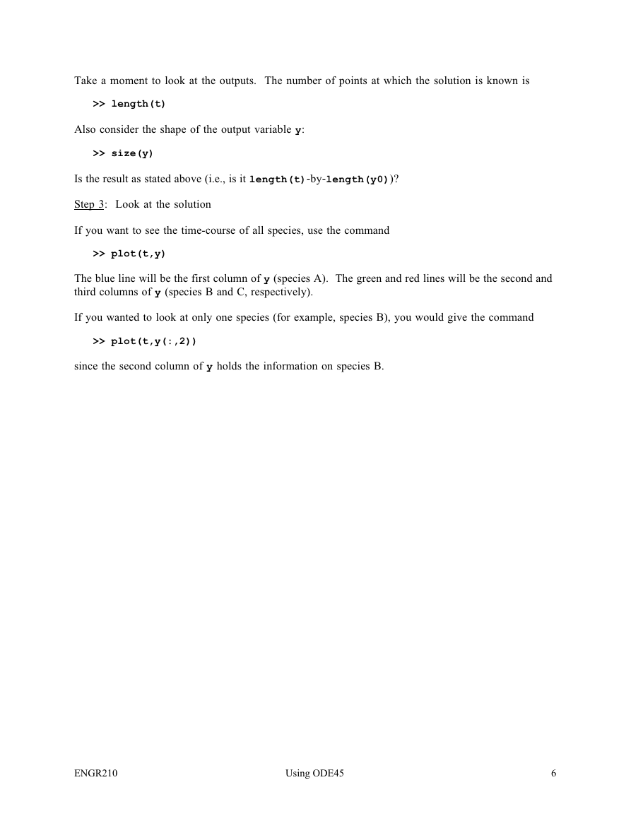
Take a moment to look at the outputs. The number of points at which the solution is known is
>> length(t)
Also consider the shape of the output variable y:
>> size(y)
Is the result as stated above (i.e., is it length(t)-by-length(y0))?
Step 3: Look at the solution
If you want to see the time-course of all species, use the command
>> plot(t,y)
The blue line will be the first column of y (species A). The green and red lines will be the second and
third columns of y (species B and C, respectively).
If you wanted to look at only one species (for example, species B), you would give the command
>> plot(t,y(:,2))
since the second column of y holds the information on species B.
ENGR210
Using ODE45
6
�
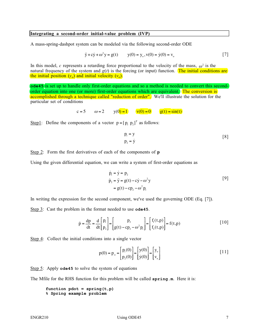
Integrating a second-order initial-value problem (IVP)
A mass-spring-dashpot system can be modeled via the following second-order ODE
+
˙˙
˙
y cy
+
ω2
y
=
( )
g t
y
( )
0
=
y v
o
, ( )
0
=
˙( )
0
y
=
v
o
[7]
In this model, c represents a retarding force proportional to the velocity of the mass, ω2 is the
natural frequency of the system and g(t) is the forcing (or input) function. The initial conditions are
the initial position (yo) and initial velocity (vo).
ode45 is set up to handle only first-order equations and so a method is needed to convert this second-
order equation into one (or more) first-order equations which are equivalent. The conversion is
accomplished through a technique called "reduction of order". We'll illustrate the solution for the
particular set of conditions
=
=
ω
=
=
=
y
0
( )
1
v
0
( )
0
c
5
2
( )
g t
sin( )
t
Step1: Define the components of a vector p = [
p p1
2
]
T as follows:
=
y
= ˙
y
p
1
p
2
Step 2: Form the first derivatives of each of the components of p
Using the given differential equation, we can write a system of first-order equations as
˙
p
1
˙
p
2
= =
= =
=
˙
y
˙˙
y
( )
g t
−
p
2
( )
g t
−
cp
2
−
˙
cy
−
ω
2
ω
2
y
p
1
In writing the expression for the second component, we've used the governing ODE (Eq. [7]).
Step 3: Cast the problem in the format needed to use ode45.
=
˙
p
=
p
d
dt
p
1
p
2
d
dt
=
p
2
cp
2
−
( )
g t
=
p
( , )
t
p
( , )
t
f
1
f
2
−
ω
2
p
1
=
f p
( , )
t
Step 4: Collect the initial conditions into a single vector
p
( )
0
=
p
o
=
p
1
p
2
( )
0
( )
0
=
( )
0
y
˙( )
0
y
=
y
v
o
o
Step 5: Apply ode45 to solve the system of equations
The Mfile for the RHS function for this problem will be called spring.m. Here it is:
function pdot = spring(t,p)
% Spring example problem
[8]
[9]
[10]
[11]
ENGR210
Using ODE45
7
�
% Parameters - damping coefficient and natural frequency
c = 5; w = 2;
g = sin(t); % forcing function
pdot = zeros(size(p));
pdot(1) = p(2);
pdot(2) = g - c*p(2) - (w^2)*p(1);
% eof - spring.m
The call to ode45 is, for a solution interval of 0 to 20,
>> p0 = [1 0];
>> [t,p] = ode45('spring',[0 20],p0);
(initial position and velocity)
Step 6: Look at the results
If you wanted to look at only the displacement, you'd want to look at the first column of p (see the
definition of p in the first step, Eq. [8]). Hence, you would give the command
>> plot(t,p(:,1))
An interesting plot for these sorts of problems is the phase-plane plot, a plot of the velocity of the
mass versus its position. This plot is easily created from your solution via
>> plot(p(:,1),p(:,2))
Phase-plane plots are useful in analyzing general features of dynamic systems.
Integrating an Nth-order initial-value problem
To use ode45 to integrate an Nth-order ODE, you simply continue the process outlined in the
section on integrating a 2nd-order ODE. The first element of the vector p is set to the dependent
variable and then subsequent elements are defined as the derivatives of the dependent variable up to
one less than the order of the equation. Finally, the initial conditions are collected into one vector
to give the format presented in Eq. [1].
For example, the 4th-order equation
a
4
d y
4
dx
+
b
3
d y
3
dx
+
c
2
d y
2
dx
+
d
dy
dx
+
ey
=
0
would generate the first-order system
d
dt
p
1
p
2
p
3
p
4
=
−
(
p
2
p
3
p
4
+
dp
2
+
ep
1
) /
a
bp
4
+
cp
3
which, along with an appropriate set of initial conditions would complete the set-up for ode45.
ENGR210
Using ODE45
[12]
[13]
8
�



 2023年江西萍乡中考道德与法治真题及答案.doc
 2012年重庆南川中考生物真题及答案.doc
 2013年江西师范大学地理学综合及文艺理论基础考研真题.doc
 2020年四川甘孜小升初语文真题及答案I卷.doc
 2020年注册岩土工程师专业基础考试真题及答案.doc
 2023-2024学年福建省厦门市九年级上学期数学月考试题及答案.doc
 2021-2022学年辽宁省沈阳市大东区九年级上学期语文期末试题及答案.doc
 2022-2023学年北京东城区初三第一学期物理期末试卷及答案.doc
 2018上半年江西教师资格初中地理学科知识与教学能力真题及答案.doc
 2012年河北国家公务员申论考试真题及答案-省级.doc
 2020-2021学年江苏省扬州市江都区邵樊片九年级上学期数学第一次质量检测试题及答案.doc
 2022下半年黑龙江教师资格证中学综合素质真题及答案.doc