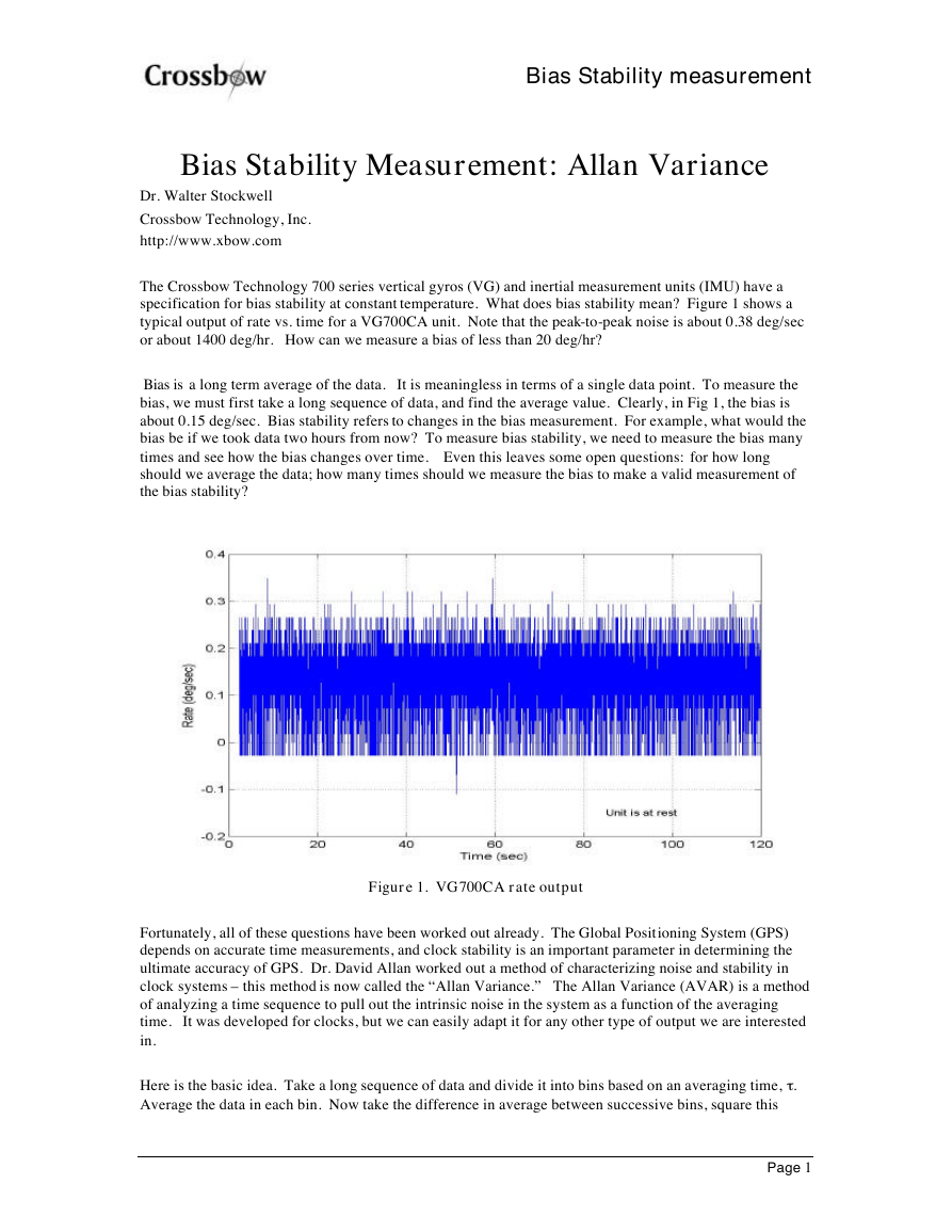
Bias Stability measurement Bias Stability Measurement: Allan Variance Dr. Walter Stockwell Crossbow Technology, Inc. http://www.xbow.com The Crossbow Technology 700 series vertical gyros (VG) and inertial measurement units (IMU) have a specification for bias stability at constant temperature. What does bias stability mean? Figure 1 shows a typical output of rate vs. time for a VG700CA unit. Note that the peak-to-peak noise is about 0.38 deg/sec or about 1400 deg/hr. How can we measure a bias of less than 20 deg/hr? Bias is a long term average of the data. It is meaningless in terms of a single data point. To measure the bias, we must first take a long sequence of data, and find the average value. Clearly, in Fig 1, the bias is about 0.15 deg/sec. Bias stability refers to changes in the bias measurement. For example, what would the bias be if we took data two hours from now? To measure bias stability, we need to measure the bias many times and see how the bias changes over time. Even this leaves some open questions: for how long should we average the data; how many times should we measure the bias to make a valid measurement of the bias stability? Figure 1. VG700CA rate output Fortunately, all of these questions have been worked out already. The Global Positioning System (GPS) depends on accurate time measurements, and clock stability is an important parameter in determining the ultimate accuracy of GPS. Dr. David Allan worked out a method of characterizing noise and stability in clock systems – this method is now called the “Allan Variance.” The Allan Variance (AVAR) is a method of analyzing a time sequence to pull out the intrinsic noise in the system as a function of the averaging time. It was developed for clocks, but we can easily adapt it for any other type of output we are interested in. 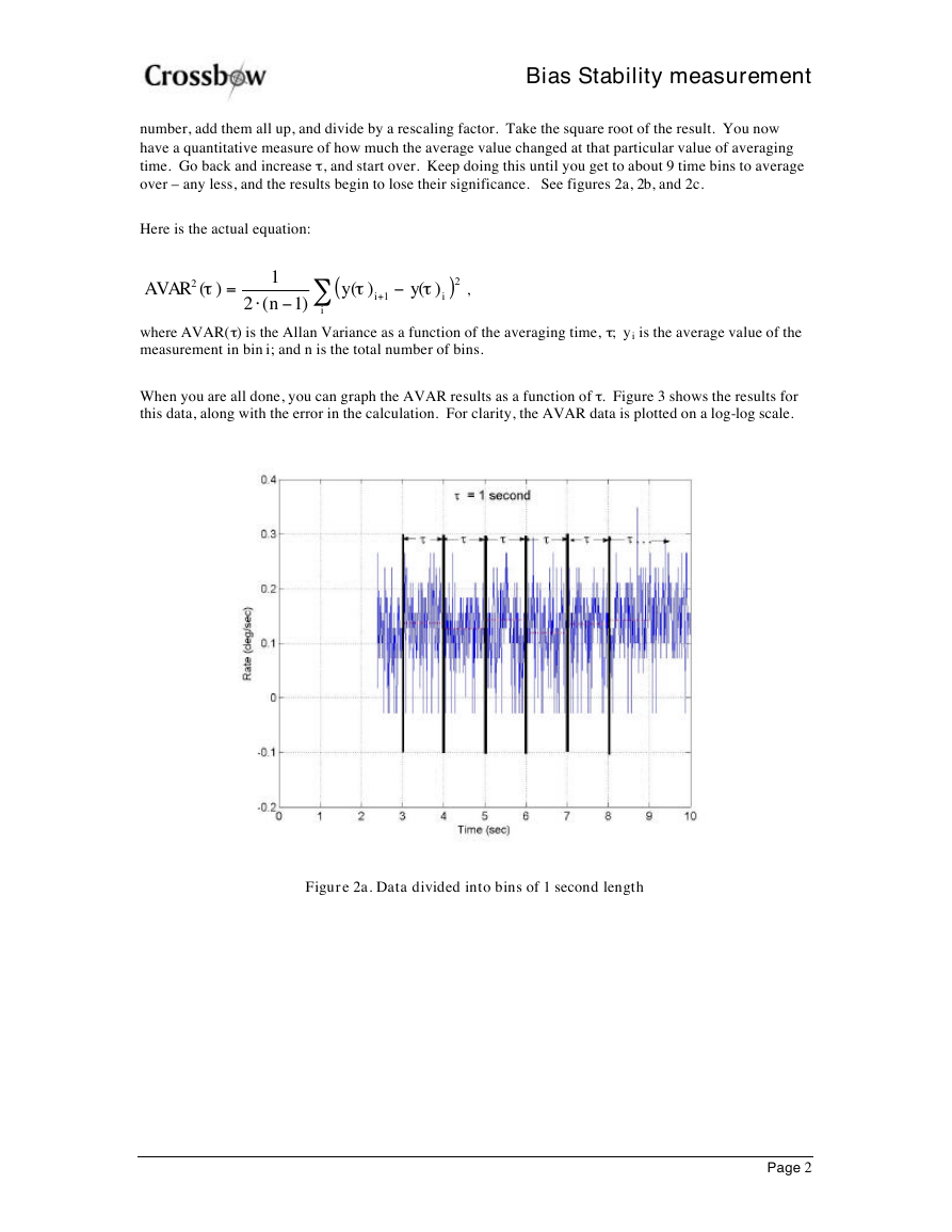Here is the basic idea. Take a long sequence of data and divide it into bins based on an averaging time, t . Average the data in each bin. Now take the difference in average between successive bins, square this Page 1 

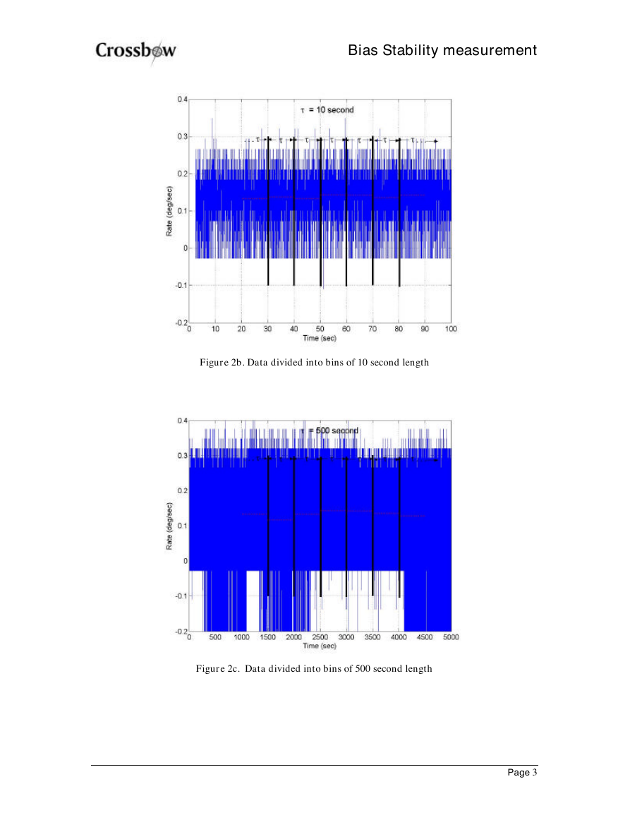
Bias Stability measurement number, add them all up, and divide by a rescaling factor. Take the square root of the result. You now have a quantitative measure of how much the average value changed at that particular value of averaging time. Go back and increase t , and start over. Keep doing this until you get to about 9 time bins to average over – any less, and the results begin to lose their significance. See figures 2a, 2b, and 2c. Here is the actual equation: AVAR 2 t )( = 1 n (2 )1 i ( y t )( + 1 i t )( y i ) 2 , where AVAR(t ) is the Allan Variance as a function of the averaging time, t ; yi is the average value of the measurement in bin i; and n is the total number of bins. 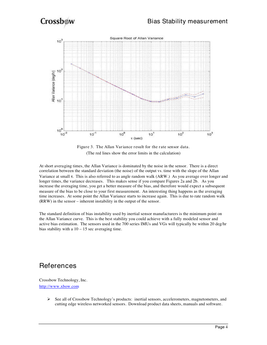When you are all done, you can graph the AVAR results as a function of t . Figure 3 shows the results for this data, along with the error in the calculation. For clarity, the AVAR data is plotted on a log-log scale. Figure 2a. Data divided into bins of 1 second length Page 2 - - 

Bias Stability measurement Figure 2b. Data divided into bins of 10 second length Figure 2c. Data divided into bins of 500 second length Page 3 

Bias Stability measurement Figure 3. The Allan Variance result for the rate sensor data. (The red lines show the error limits in the calculation) At short averaging times, the Allan Variance is dominated by the noise in the sensor. There is a direct correlation between the standard deviation (the noise) of the output vs. time with the slope of the Allan Variance at small t . This is also referred to as angle random walk (ARW.) As you average over longer and longer times, the variance decreases. This makes sense if you compare Figures 2a and 2b. As you increase the averaging time, you get a better measure of the bias, and therefore would expect a subsequent measure of the bias to be close to your first measurement. An interesting thing happens as the averaging time increases. At some point the Allan Variance starts to increase again. This is due to rate random walk (RRW) in the sensor – inherent instability in the output of the sensor. The standard definition of bias instability used by inertial sensor manufacturers is the minimum point on the Allan Variance curve. This is the best stability you could achieve with a fully modeled sensor and active bias estimation. The sensors used in the 700 series IMUs and VGs will typically be within 20 deg/hr bias stability with a 10 – 15 sec averaging time. References Crossbow Technology, Inc. http://www.xbow.com See all of Crossbow Technology’s products: inertial sensors, accelerometers, magnetometers, and cutting edge wireless networked sensors. Download product data sheets, manuals and software. Page 4 

Dr. David Allan’s website about Allan Variance Calculations. http://www.allanstime.com/AllanVariance/index.html Bias Stability measurement This website is a good place to start in understanding the Allan Variance. He has equations, a good explanation, and links to applications and technical discussions. IEEE Std 952-1997, "Guide and Test Procedure for Single Axis Interferometric Fiber Optic Gyros," IEEE, 1997, p.63. IEEE standard for defining methods to characterize FOG sensors. Includes a long appendix describing the Allan Variance measurement in more detail. Page 5