雅可比矩阵逆解.pdf

发布时间：2022-06-10 发布人：admin 分类：说明书资料大小：1.52M 资料格式：pdf 举报版权申诉

baidu_36487340-11953096-16359648084670860158.pdf-第1页.png

第1页 / 共23页

baidu_36487340-11953096-16359648084670860158.pdf-第2页.png

第2页 / 共23页

baidu_36487340-11953096-16359648084670860158.pdf-第3页.png

第3页 / 共23页

baidu_36487340-11953096-16359648084670860158.pdf-第4页.png

第4页 / 共23页

baidu_36487340-11953096-16359648084670860158.pdf-第5页.png

第5页 / 共23页

baidu_36487340-11953096-16359648084670860158.pdf-第6页.png

第6页 / 共23页

baidu_36487340-11953096-16359648084670860158.pdf-第7页.png

第7页 / 共23页

baidu_36487340-11953096-16359648084670860158.pdf-第8页.png

第8页 / 共23页

文本预览

Jacobian methods for inverse kinematics and planning Slides from Stefan Schaal USC, Max Planck

The Inverse Kinematics Problem   Direct Kinematics   Inverse Kinematics x = f θ( ) θ= f −1 x( )   Possible Problems of Inverse Kinematics Infinitely many solutions   Multiple solutions     No solutions   No closed-form (analytical solution)

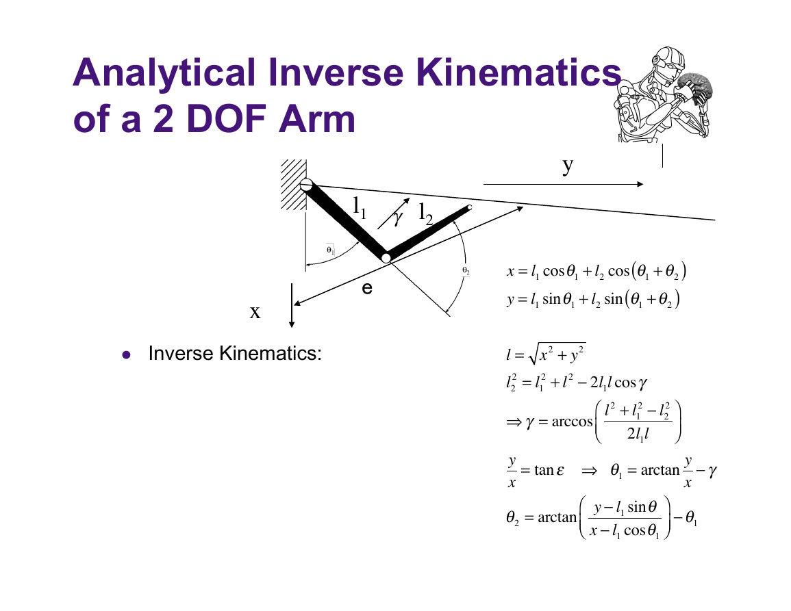
Analytical (Algebraic) Solutions   Analytically invert the direct kinematics equations and enumerate all solution branches   Note: this only works if the number of constraints is the same as the number of degrees-of-freedom of the robot   What if not?     Iterative solutions Invent artificial constraints   Examples   2DOF arm   See S&S textbook 2.11 ff

Analytical Inverse Kinematics of a 2 DOF Arm y l1 l2 γ e x   Inverse Kinematics: x = l1 cosθ1 + l2 cos θ1 +θ2 y = l1 sinθ1 + l2 sin θ1 +θ2 ) ( ( ) ⎛ ⎝⎜ l = x2 + y2 2 + l2 − 2l1lcosγ l2 2 = l1 ⇒γ = arccos l2 + l1 2 − l2 2 ⎞ 2l1l ⎠⎟ y x = tanε ⇒ θ1 = arctan y ⎞ θ2 = arctan ⎠⎟ −θ1 y − l1 sinθ x − l1 cosθ1 x −γ ⎛ ⎝⎜

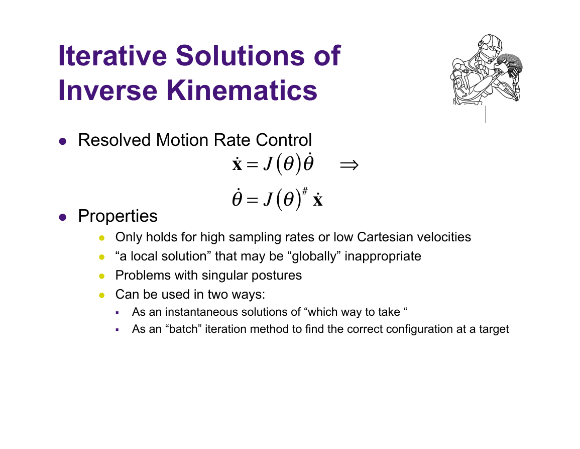
Iterative Solutions of Inverse Kinematics   Resolved Motion Rate Control x = J θ( ) θ ⇒ θ= J θ( )# x   Properties   Only holds for high sampling rates or low Cartesian velocities   “a local solution” that may be “globally” inappropriate   Problems with singular postures   Can be used in two ways:   As an instantaneous solutions of “which way to take “   As an “batch” iteration method to find the correct configuration at a target

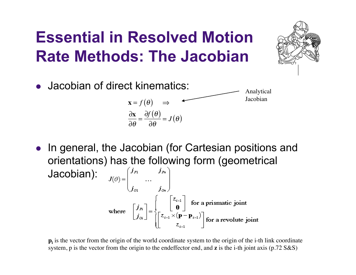
Essential in Resolved Motion Rate Methods: The Jacobian   Jacobian of direct kinematics: x = f θ( ) ⇒ ∂x ∂θ ∂f θ( ) ∂θ = = J θ( ) Analytical Jacobian   In general, the Jacobian (for Cartesian positions and orientations) has the following form (geometrical Jacobian): pi is the vector from the origin of the world coordinate system to the origin of the i-th link coordinate system, p is the vector from the origin to the endeffector end, and z is the i-th joint axis (p.72 S&S)

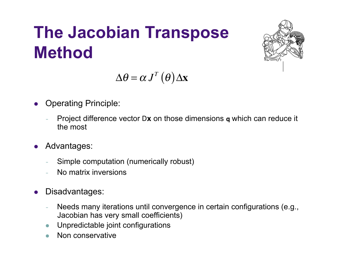
The Jacobian Transpose Method Δθ=αJ T θ( )Δx   Operating Principle: -  Project difference vector Dx on those dimensions q which can reduce it the most   Advantages: -  Simple computation (numerically robust) -  No matrix inversions   Disadvantages: -  Needs many iterations until convergence in certain configurations (e.g., Jacobian has very small coefficients)   Unpredictable joint configurations   Non conservative

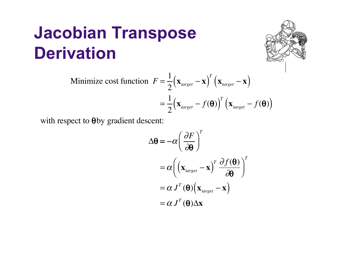
Jacobian Transpose Derivation Minimize cost function F = = with respect to θ by gradient descent: 1 ( )T xtarget − x ( 2 xtarget − x 1 ( 2 xtarget − f (θ) ) )T xtarget − f (θ) ( ) Δθ = −α ∂F ∂θ T ⎞ ⎠⎟ ⎛ ⎝⎜ ( T ⎞ ⎠⎟ ⎛ ⎝⎜ )T ∂f (θ) =α xtarget − x ∂θ ( ) =αJ T (θ) xtarget − x =αJ T (θ)Δx

分享到：

赞收藏

资料库

雅可比矩阵逆解.pdf

相关推荐

课程资源

热门标签

最新资料