IEEE TRANSACTIONS ON PATTERN ANALYSIS AND MACHINE INTELLIGENCE. VOL. 11. NO
I?. DECEMBER 198’)
1293
Subpixel Measurements Using a Moment-Based Edge
Operator
EDWARD P. LYVERS, OWEN ROBERT MITCHELL, SENIOR MEMBER, IEEE,
MARK L. AKEY, MEMBER, IEEE, AND ANTHONY P. REEVES, SENIOR MEMBER, IEEE
Abstract-This paper presents recent results in precision measure-
ments using computer vision. An edge operator based on two-dimen-
sional spatial moments is presented. The operator can be implemented
for virtually any size window and has been shown to locate edges in
digitized images to a twentieth of a pixel. This accuracy is unaffected
by additive or multiplicative changes to the data values. The precision
is achieved by correcting for many of the deterministic errors caused
by nonideal edge profiles using a look-up table to correct the original
estimates of edge orientation and location. This table is generated using
a synthesized edge which is located at various subpixel locations and
various orientations. The operator is extended to accommodate non-
ideal edge profiles and rectangularly sampled pixels. The application
of this technique to the measurement of imaged machined metal parts
is also presented. Additionally, both theortical and experimental noise
analyses show the operator has a relatively small bias in the presence
of noise.
Index Terms-Edge detection, edge location, facet model, Hueckel,
image processing, Laplacian of a Gaussian, spatial moments, subpixel
measurement.
U agery to within a pixel has seemed adequate. For
NTIL recently, the location of features in digital im-
I. INTRODUCTION
those cases which require higher precision, the primary
solution has been to increase the sampling rate. However,
there are applications in the digital image processing field
that need better accuracy. These include photogrammetry
and industrial inspection, where measurement accuracy is
at a premium.
Up to this point few edge locators have been capable of
subpixel accuracy. Frei and Chen [l], Roberts [2], and
Sobel [3] have all proposed edge detection schemes which
use some digital approximation to the gradient. These
methods are very fast and deliver acceptable results; how-
ever, the locations are not subpixel and the derivative op-
eration is very sensitive to noise. Macvicar-Whelan and
Binford [4] have proposed a method which utilizes the
gradient operation after the data has been smoothed within
an arbitrary odd-sized window. The subpixel edge loca-
Manuscript received September 30, 1984; revised July 20, 1989. Rec-
Wayne, IN 46808.
versity, Ithaca, NY 14853.
IEEE Log Number 893 11 17.
ommended for acceptance by W. E. L. Grimson.
E. P. Lyvers is with MIT Lincoln Laboratory, Lexington, MA 01273.
0. R. Mitchell is with the Department of Electrical Engineering, Uni-
versity of Texas at Arlington, Arlington, TX 76019.
M. L. Akey is with Magnavox Electronics System Company, Fort
A. P. Reeves is with the School of Electrical Engineering, Cornel1 Uni-
tions are determined by linearly interpolating the location
within a rise-fall-rise region of the gradient. This method
is much less sensitive to noise in comparison to the other
gradient operators; however, precision is limited to inter-
polation between a few points. Machuca and Gilbert [5]
have proposed a method which integrates the region con-
taining the edge. This method uses the moments found in
the region to determine the position of the edge. Nevatia
and Babu [6] have designed a linear feature extractor using
edge detection and line thinning. Their edge detector con-
volves windowed data with six edge masks. The maxi-
mum response from this matched filter is chosen as the
correct edge orientation of an edge centered in the win-
dow. Hueckel [7]-[9] has developed an algorithm to de-
termine the presence of edges and lines by fitting a region
of data to a Hilbert space with 9 parameters. The locations
are to subpixel accuracies; however, no analysis of the
operator in the presence of noise is documented. Tabata-
bai and Mitchell [lo] have developed an operator which
locates edges by fitting the first three gray level moments
to the data. Again, the edge locations are to subpixel ac-
curacies as well as being much less sensitive to noise when
compared to the Hueckel operator. Huertas and Medioni
[ l 11 have developed a subpixel operator using the facet
model combined with Laplacian of Gaussian masks. Eng-
lander [12] describes a subpixel operator based on image
resampling using Whittaker’s theorem.
This paper presents a new edge operator (detector)
which uses the spatial moments of a gray level edge to
determine the location of the edge. Section I1 defines the
one-dimensional edge operator. The operator is evaluated
for subpixel accuracy as well as performance in the pres-
ence of noise. The Tabatabai operator is implemented in
one dimension and compared to the moment based edge
operator. Section I11 defines the two-dimensional edge op-
erator. Again, the operator is tested for subpixel accuracy
in addition to performance in the presence of noise. The
Tabatabai, the Hueckel, and a modified version of the
Huertas and Medioni edge operators are compared to the
moment based edge operator. A confidence measure is de-
veloped for the two-dimensional operator. In addition, re-
cent tests of the method on precision edge contrast and
orientation estimation [ 131 show this new moment method
to outperform Sobel, Nevatia-Babu, facet model, and
Gaussian smoothed gradient techniques.
0162-8828/89/1200-1293$01 .OO 0 1989 IEEE
Authorized licensed use limited to: Wuhan University. Downloaded on April 24,2010 at 02:57:08 UTC from IEEE Xplore. Restrictions apply.
�
1294
IEEE TRANSACTIONS ON PATTERN ANALYSIS AND MACHINE INTELLIGENCE. VOL. 1 1 . NO. I?. DECEMBER 1989
11. ONE-DIMENSIONAL EDGE OPERATOR
The new edge operator uses the spatial moments of the
discrete edge data to determine the position of an edge.
The moments of an ideal edge in a continuous domain are
determined and the position of the edge is mathematically
derived from these moments. The position results are then
modified to correct for deterministic errors due to the
sampling. The edge operator is then applied to noisy data.
Theoretical and empirical statistics are determined.
Lastly, a one-dimensional gray level moment edge oper-
ator developed by Tabatabai and Mitchell [lo] is imple-
mented and its performance is compared to the spatial
moment edge operator results.
A. Derivation of the One-Dimensional Edge Operator
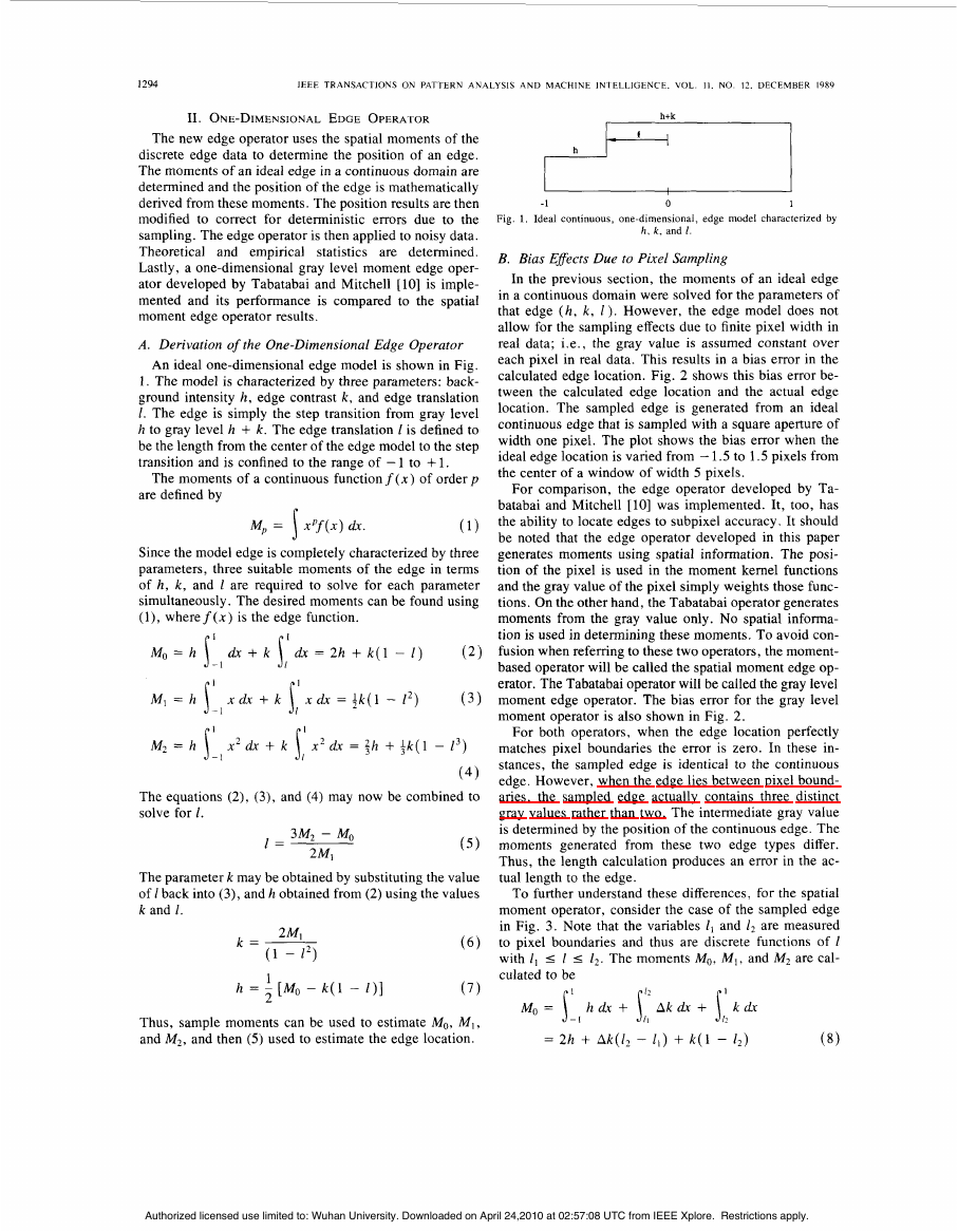
An ideal one-dimensional edge model is shown in Fig.
1. The model is characterized by three parameters: back-
ground intensity h, edge contrast k, and edge translation
1. The edge is simply the step transition from gray level
h to gray level h + k. The edge translation 1 is defined to
be the length from the center of the edge model to the step
transition and is confined to the range of - 1 to + 1.
The moments of a continuous functionf(x) of order p
are defined by
Mp = 1 x p f ( x ) ah.
(1)
Since the model edge is completely characterized by three
parameters, three suitable moments of the edge in terms
of h, k, and 1 are required to solve for each parameter
simultaneously. The desired moments can be found using
(l), where f (x) is the edge function.
MO = h i l l a h + k ! ‘ a h = 2h + k(l - I )
MI = h 1 x d x + k [ ah = ik(l - 1’)
M2 = h 1’ x 2 a h + k 1 ’ x 2 a h = j h + ik(1 - 1 3 )
-1
1
1
1
I
I
- I
h+k
I
-1
0
1
1
Fig. 1, Ideal continuous, one-dimensional, edge model characterized by
h , k , and 1.
B. Bias Efects Due to Pixel Sampling
In the previous section, the moments of an ideal edge
in a continuous domain were solved for the parameters of
that edge ( h , k, 1). However, the edge model does not
allow for the sampling effects due to finite pixel width in
real data; i.e., the gray value is assumed constant over
each pixel in real data. This results in a bias error in the
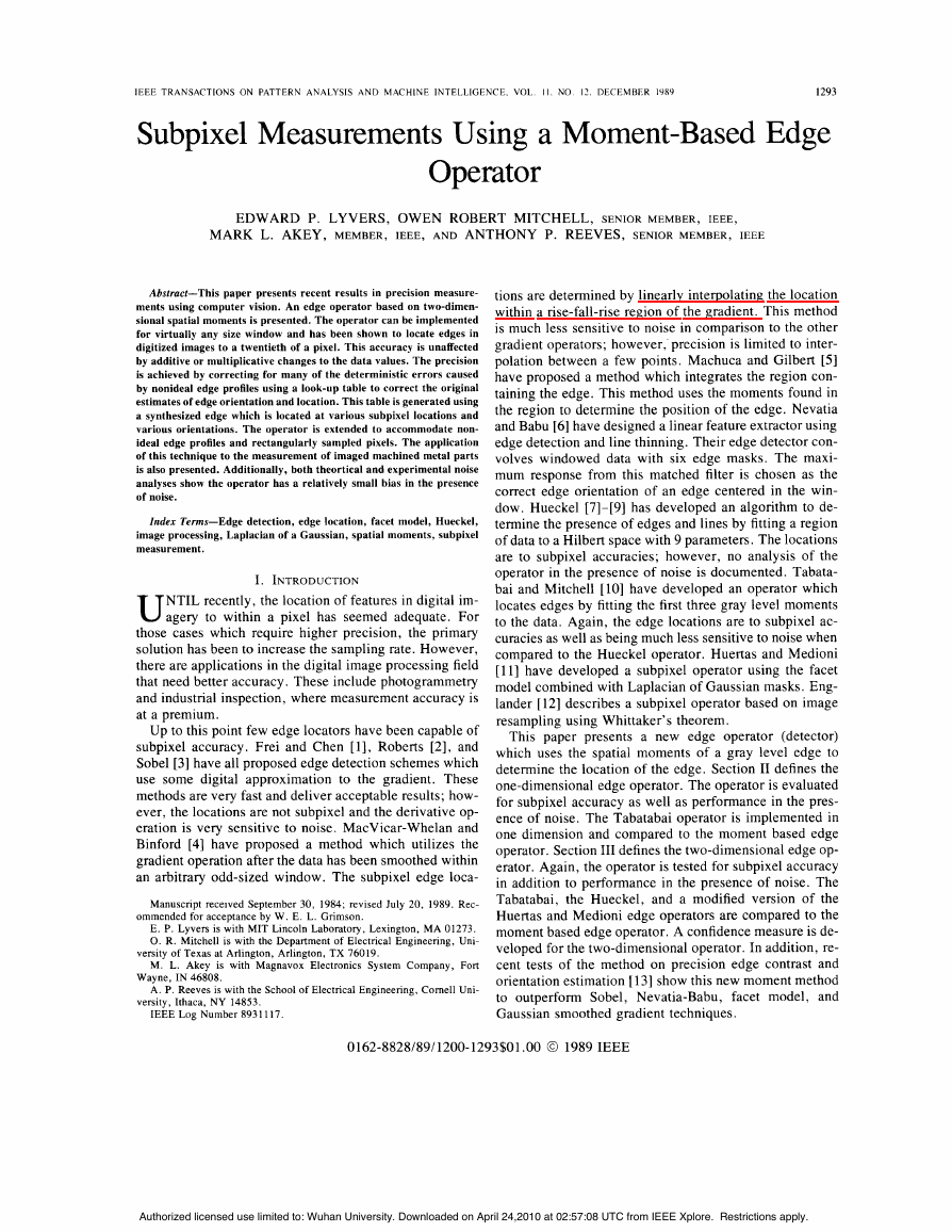
calculated edge location. Fig. 2 shows this bias error be-
tween the calculated edge location and the actual edge
location. The sampled edge is generated from an ideal
continuous edge that is sampled with a square aperture of
width one pixel. The plot shows the bias error when the
ideal edge location is vaned from - 1.5 to 1.5 pixels from
the center of a window of width 5 pixels.
For comparison, the edge operator developed by Ta-
batabai and Mitchell [lo] was implemented. It, too, has
the ability to locate edges to subpixel accuracy. It should
be noted that the edge operator developed in this paper
generates moments using spatial information. The posi-
tion of the pixel is used in the moment kernel functions
and the gray value of the pixel simply weights those func-
tions. On the other hand, the Tabatabai operator generates
moments from the gray value only. No spatial informa-
tion is used in determining these moments. To avoid con-
fusion when refemng to these two operators, the moment-
based operator will be called the spatial moment edge op-
erator. The Tabatabai operator will be called the gray level
moment edge operator. The bias error for the gray level
moment operator is also shown in Fig. 2 .
For both operators, when the edge location perfectly
matches pixel boundaries the error is zero. In these in-
stances, the sampled edge is identical to the continuous
edge. However, when the edge lies between pixel bound-
aries, the sampled edge actually contains three distinct
gray values rather than two. The intermediate gray value
is determined by the position of the continuous edge. The
moments generated from these two edge types differ.
Thus, the length calculation produces an error in the ac-
tual length to the edge.
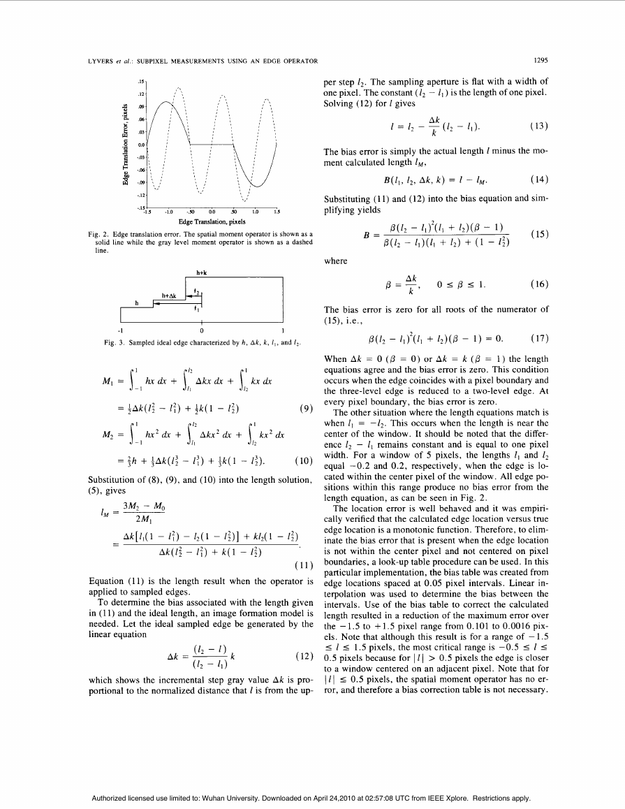
To further understand these differences, for the spatial
moment operator, consider the case of the sampled edge
in Fig. 3 . Note that the variables lI and l2 are measured
to pixel boundaries and thus are discrete functions of I
with l1 I 1 I 12. The moments MO, MI, and M2 are cal-
culated to be
M O = j l l h a k + j
= 2h + Ak(Z2 - 11) + k( 1 - Z2)
II A k d x + j ’ k d x
IZ
12
( 8 )
( 2 )
( 3 )
(4)
The equations (2), ( 3 ) , and (4) may now be combined to
solve for 1.
( 5 )
The parameter k may be obtained by substituting the value
of 1 back into ( 3 ) , and h obtained from ( 2 ) using the values
k and 1.
Thus, sample moments can be used to estimate MO, M I ,
and M2, and then (5) used to estimate the edge location.
Authorized licensed use limited to: Wuhan University. Downloaded on April 24,2010 at 02:57:08 UTC from IEEE Xplore. Restrictions apply.
�
LYVERS er al.: SUBPIXEL MEASUREMENTS USING AN EDGE OPERATOR
1295
per step 1,. The sampling aperture is flat with a width of
one pixel. The constant ( l2 - l1 ) is the length of one pixel.
Solving (12) for 1 gives
1 = 12 - - ( & - 1 1 ) .
Ak
k
(13)
The bias error is simply the actual length 1 minus the mo-
ment calculated length l,,.,,
B ( l l , 12, Ak, k) = 1 - 1M.
(14)
Substituting (1 1) and (12) into the bias equation and sim-
plifying yields
where
p = -
Ak
k '
o r p 5 1 .
(16)
The bias error is zero for all roots of the numerator of
(13, i.e.,
P(1, - 11)2(Z, + 1 2 ) ( P - 1 ) = 0.
(17)
When Ak = 0 (0 = 0 ) or Ak = k (0 = 1 ) the length
equations agree and the bias error is zero. This condition
occurs when the edge coincides with a pixel boundary and
the three-level edge is reduced to a two-level edge. At
every pixel boundary, the bias error is zero.
The other situation where the length equations match is
when l1 = -12. This occurs when the length is near the
center of the window. It should be noted that the differ-
ence l2 - Zl remains constant and is equal to one pixel
width. For a window of 5 pixels, the lengths lI and 1,
equal -0.2 and 0.2, respectively, when the edge is lo-
cated within the center pixel of the window. All edge po-
sitions within this range produce no bias error from the
length equation, as can be seen in Fig. 2.
The location error is well behaved and it was empiri-
cally verified that the calculated edge location versus true
edge location is a monotonic function. Therefore, to elim-
inate the bias error that is present when the edge location
is not within the center pixel and not centered on pixel
boundaries, a look-up table procedure can be used. In this
particular implementation, the bias table was created from
edge locations spaced at 0.05 pixel intervals. Linear in-
terpolation was used to determine the bias between the
intervals. Use of the bias table to correct the calculated
length resulted in a reduction of the maximum error over
the -1.5 to +1.5 pixel range from 0.101 to 0.0016 pix-
els. Note that although this result is for a range of - 1.5
I Z I 1.5 pixels, the most critical range is -0.5 I 1 I
0.5 pixels because for I 1 I > 0.5 pixels the edge is closer
to a window centered on an adjacent pixel. Note that for
1 1 I I 0.5 pixels, the spatial moment operator has no er-
ror, and therefore a bias correction table is not necessary.
-1.5
-1.0
-.50
0.0
.50
1.0
1.5
Edge Translation, pixels
Fig. 2. Edge translation error. The spatial moment operator is shown as a
solid line while the gray level moment operator is shown as a dashed
line.
h+k
-1
0
1
Fig. 3. Sampled ideal edge characterized by h, Ak, k, l , , and 12.
M~ = 1 hx2 dr + A,,
Akx'dr + J,, kx2
= $h + fAk(1; - I:) + fk( 1 - 1;).
- 1
(10)
Substitution of (8), (9), and (IO) into the length solution,
( 5 ) , gives
I,,., =
3M2 - MO
2Ml
- -
Ak[ZI(l - 1:) - 12(1 - l ; ) ] + k12(1 - 1:)
Ak(1: - 1:) + k( 1 - 1;)
(11)
Equation (11) is the length result when the operator is
applied to sampled edges.
To determine the bias associated with the length given
in (1 1) and the ideal length, an image formation model is
needed. Let the ideal sampled edge be generated by the
linear equation
which shows the incremental step gray value Ak is pro-
portional to the normalized distance that 1 is from the up-
Authorized licensed use limited to: Wuhan University. Downloaded on April 24,2010 at 02:57:08 UTC from IEEE Xplore. Restrictions apply.
�
~
1296
JEEE TRANSACTIONS ON PATTERN ANALYSIS AND MACHlNE INTELLIGENCE. VOL. I I . NO. 12. DECEMBER 1989
Other effects may also be incorporated into the error
bias table. For instance, the sampling effects caused by a
Gaussian-type aperture, rather than the square aperture
used here, could be accounted for in the bias table. Non-
symmetric edges which are caused by cylindrical surfaces
can also be located precisely with the bias table. How-
ever, this requires the nonsymmetric edge to be well mod-
eled so that the appropriate bias table may be determined.
Three-Level Model: Some thought has been directed
toward establishing the three gray level edge as an edge
model and finding the solution for the length using the
new model’s moments. In this implementation, the length
solution would not be in error. However, due to the in-
creased complexity of the edge model, five parameters are
needed to describe it sufficiently. The five parameters are
h, Ak, k , 1 1 , and 1,. If the operator is applied only to edges
blurred over one pixel, l2 - II will be known. Therefore,
the first four moments of the edge need to be calculated
and solved for h, Ak, k , I,, and 12. The solution, however,
is not readily apparent. The additional length variable in-
creases the complexity, prohibiting a closed form solu-
tion. For this reason, the three level edge model is dropped
in favor of the original edge model.
The location error for the gray level operator was also
well behaved and a look-up table procedure was used for
it too. The bias table was created from edge locations
spaced at 0.05 pixel intervals. Use of the bias table to
correct the calculated length resulted in a reduction of the
maximum error over the - 1.5 to + 1.5 pixel range from
0.136 to 0.045 pixels.
C. Efects of Noise on Edge Location
The effects of noise on the edge location determined by
the operator will now be considered. The bias correction
is not considered in the theoretical noise analysis. Incor-
porating the correction given in (15) into a noise model
would complicate the analysis significantly.
Assume additive, independent, identically distributed,
Gaussian noise is added to the pixel gray values of a sam-
pled ideal edge. The calculated length ( 5 ) now becomes
a random variable, i.e.,
Analysis is simplified if the length is considered to be the
quotient of two random variables, gN and go, such that
gN = 3m, - mo and go = 2ml.
(19)
The moments of a discrete function f ( i ) are given by
Mp = .x c p ( i > f ( i )
K
r = l
are given by
mp = c c , ( i ) [ f ( i ) + rqi)]
K
i = I
K
K
= C c , ( i > f ( i > + C c,(i) A ( i )
= M, + rip.
i = I
r = I
(22)
The random moment, therefore, can be viewed as a de-
terministic part plus a random part. Furthermore, li,
is
simply the weighted sum of K independent, zero-mean
Gaussian random variables. The resulting random vari-
able ti,, is Gaussian distributed and is well documented in
the literature [ 141.
In the case where K is of moderate value, the distribu-
tion of each A ( i ) need not even be Gaussian, but only
reasonably concentrated about the mean. This condition
stems from the well known central-limit theorem. The
mean of the resulting Gaussian density is zero and the
variance is the sum of variances from each random vari-
able. Each individual variance is the weighted variance of
the additive noise, i.e.,
a i p = [c;(l) + * . * + c ; ( K ) ] a 2
(23)
where is2 is the variance of the additive noise. For a win-
dow size of 5 pixels the numerator and denominator stan-
dard deviations are
oN = 0.71840 and aD = 1.01190.
(24)
The Gaussian random variables gN and go can now be pa-
rameterized,
giy = 3(M2 f A 2 ) - (MO + A())
= 3M2 - MO f 3A2 - fio
where
and
where
c1.N = 3M2 - MO
0; = a2 r = l c [3c2(i) - co(i)12
K
go = 2(M, + A , ) = 2M1 + 2Al
P D = 2M1
K
(25)
(26)
(27)
(28)
(29)
where c, ( i ) is the pth order moment weighting for the
pixel region indicated by i. The moments from a sampled,
noisy edge,
f ( i ) = f ( i ) + a ( i )
(20)
The random length (1 8) can now be viewed as the quo-
tient of two, nonzero mean Gaussian random variables.
To completely parameterize this relationship, the covari-
ance between the numerator and denominator random
variables must be determined. The summation of (20) can
be viewed as the inner product of a row and a column
vector. The numerator and denominator random variables
Authorized licensed use limited to: Wuhan University. Downloaded on April 24,2010 at 02:57:08 UTC from IEEE Xplore. Restrictions apply.
�
LYVERS et al.: SUBPIXEL MEASUREMENTS USING AN EDGE OPERATOR
1297
can be modeled as
g N = dTR + b,
where
= CTR + d
( 3 1 )
where
erf (x) = - exp ( - y 2 / 2 ) dy.
l s ’
O
G
* , 3 C 2 ( k ) - cO(k)]
* , 2 c l ( k ) ]
d T = [3c2( 1) - CO( l ) , . *
C T = [ 2 c l ( l ) , *
RT = [ R ( l ) , R ( 2 ) , * . * , f i ( k ) ]
b = 3Mz - MO
d = 2M1.
The expectation of gNgD is
E { g N g D } = E ( ( d T R + b)(E‘.f + d ) }
= E{nT2i;‘Z + dn’f + bcT.f + b d }
= E { d T f X T C } + bd
= d T E { R . f T } E + bd
= d T C a i + bd.
The covariance is given by
( 3 2 )
( g N g D ) = E ( g N g D } - E { g N } E( gD}
= ~ ‘ C U ; + bd - bd = ~‘CO:.
( 3 3 )
Since the moment weightings are implemented using a
symmetrical window centered at zero,
is even-valued
and C is odd-valued. Thus, their inner product, dTC, is
zero. If the two Gaussian variables are uncorrelated, then
they are necessarily independent. Therefore, the length
equation is the quotient of two nonzero independent
Gaussian random variables. For the special case when
each random variable has zero mean, the random variable
f i s Cauchy. This case arises only when the deterministic
part of the window input is a flat field of zeros. In general,
however, both random variables have nonzero mean.
A closed form solution of the density function for the
length variable does not exist. An integral form of the
density [14] has the form
IYI
(34)
It should be noted that the means of the Gaussian random
variables are determined by the actual position of the edge,
1. After a fair amount of mathematical manipulation, the
above integral can be expressed in terms of an error func-
tion as
Note that if ,uN = pD = 0 the above density reduces to a
Cauchy density as would be expected.
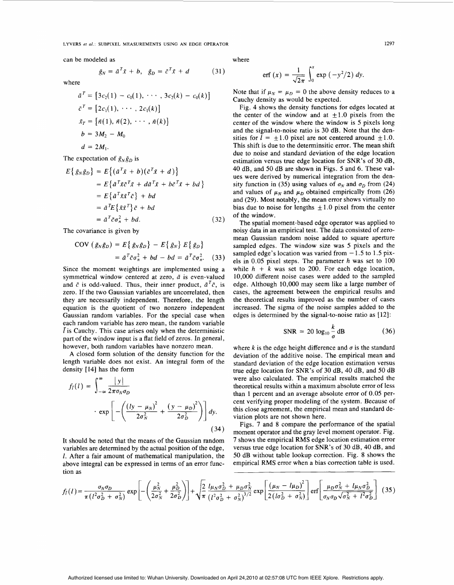
Fig. 4 shows the density functions for edges located at
the center of the window and at f 1 .O pixels from the
center of the window where the window is 5 pixels long
and the signal-to-noise ratio is 30 dB. Note that the den-
sities for 1 = +_ 1 .O pixel are not centered around * 1 .O.
This shift is due to the determinsitic error. The mean shift
due to noise and standard deviation of the edge location
estimation versus true edge location for SNR’s of 30 dB,
40 dB, and 50 dB are shown in Figs. 5 and 6 . These val-
ues were derived by numerical integration from the den-
sity function in (35) using values of uN and uD from (24)
and values of pN and pD obtained empirically from (26)
and (29). Most notably, the mean error shows virtually no
1 .O pixel from the center
bias due to noise for lengths
of the window.
The spatial moment-based edge operator was applied to
noisy data in an empirical test. The data consisted of zero-
mean Gaussian random noise added to square aperture
sampled edges. The window size was 5 pixels and the
sampled edge’s location was vaned from - 1.5 to 1.5 pix-
els in 0.05 pixel steps. The parameter h was set to 100
while h + k was set to 200. For each edge location,
10,000 different noise cases were added to the sampled
edge. Although 10,000 may seem like a large number of
cases, the agreement between the empirical results and
the theoretical results improved as the number of cases
increased. The sigma of the noise samples added to the
edges is determined by the signal-to-noise ratio as [ 121 :
SNR
20 log10 - dB
k
U
( 3 6 )
where k is the edge height difference and U is the standard
deviation of the additive noise. The empirical mean and
standard deviation of the edge location estimation versus
true edge location for SNR’s of 30 dB, 40 dB, and 50 dB
were also calculated. The empirical results matched the
theoretical results within a maximum absolute error of less
than 1 percent and an average absolute error of 0.05 per-
cent verifying proper modeling of the system. Because of
this close agreement, the empirical mean and standard de-
viation plots are not shown here.
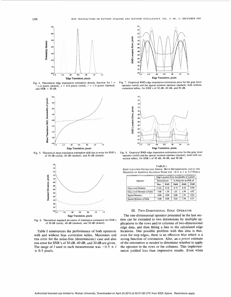
Figs. 7 and 8 compare the performance of the spatial
moment operator and the gray level moment operator. Fig.
7 shows the empirical RMS edge location estimation error
versus true edge location for SNR’s of 30 dB, 40 dB, and
50 dB without table lookup correction. Fig. 8 shows the
empirical RMS error when a bias correction table is used.
Authorized licensed use limited to: Wuhan University. Downloaded on April 24,2010 at 02:57:08 UTC from IEEE Xplore. Restrictions apply.
�
1298
lEEE TRANSACTIONS ON PATTERN ANALYSIS AND MACHINE INTELLIGENCE. VOL.
I I . NO. 12. DECEMBER 1989
7.0
6.0]
1
Edge Translation, pixels
0.0 -1.5 4
-1.0
-.M I
0.0
.M
1.0
Edge Translation, pixels
1.5 ,
Fig. 4. Theoretical edge translation estimation density function for 1 =
-1.0 pixels (dotted), 1 = 0.0 pixels (solid), 1 = 1.0 pixels (dashed),
and SNR = 30 dB.
Fig. 7. Empirical RMS edge translation estimation error for the gray level
operator (solid) and the spatial moment operator (dashed), both without
correction tables, for SNR's of 30 dB, 40 dB, and 50 dB.
-Y
-3.0
4.0 J
-1.5
-1.0
-.M
0.0
.M
1.0
1.5
Edge Translation, pixels
Fig. 5. Theoretical mean translation estimation shift due to noise for SNR's
of 30 dB (solid), 40 dB (dashed), and 50 dB (dotted).
.I4 -
.13-
3
3
m
::
.rn..-..-
.m
.01-
0.0
1
- _
- _
---..~..._....._.-
_ _ - -
Table I summarizes the performance of both operators
with and without bias correction tables. Maximum and
rms error for the noise-free (deterministic) case and also
rms error for SNR's of 50 dB, 40 dB, and 30 dB are given.
The range of I used in each measurement was -0.5 I I
I 0.5 pixels.
Edge Translation, pixels
Fig. 8. Empirical RMS edge translation estimation error for the gray level
operator (solid) and the spatial moment operator (dashed), both with cor-
rection tables, for SNR's of 30 dB, 40 dB, and 50 dB.
EDGE LOCATION ESTIMATION ERROR, BOTH DETERMINISTIC
AND IN THE
PRESENCE OF ADDITIVE GAUSSIAN NOISE FOR -0.5 I 1 I 0.5 PIXELS
TABLE I
I
Operator
Gray Level Moment
Gray Level Moment w/Table
Spatial Moment
1 Edge Location Error (hundredths of a pixel) I
In Noise for an SNR of
50dB 4OdB
30dB
I 8.90
I 8.25
1.94 4.07
1.91
6.04
Deterministic
Max
RMS
11.62 I 8.18
3.66
1.56
0.00
0.00
8.19
1.61
0.60
111. TWO-DIMENSIONAL EDGE OPERATOR
The one-dimensional operator presented in the last sec-
tion can be extended to two dimensions by multiple ap-
plications to the rows and/or columns of two-dimensional
edge data, and then fitting a line to the calculated edge
locations. One possible problem with this idea is that,
even for step edges, there is an effective blur which is a
strong function of orientation. Also, an a priori estimate
of the orientation is needed to determine whether to apply
the operator to the rows or the columns. This implemen-
tation yielded less than impressive results. Even when
Authorized licensed use limited to: Wuhan University. Downloaded on April 24,2010 at 02:57:08 UTC from IEEE Xplore. Restrictions apply.
�
LYVERS et al.: SUBPIXEL MEASUREMENTS USING A N EDGE OPERATOR
1299
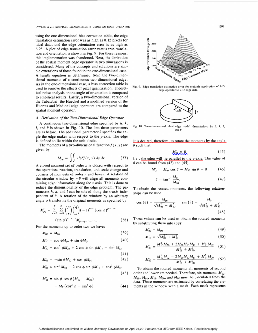
using the one-dimensional bias correction table, the edge
translation estimation error was as high as 0.12 pixels for
ideal data, and the edge orientation error is as high as
6.2". A plot of edge translation error versus true transla-
tion and orientation is shown in Fig. 9. For these reasons,
this implementation was abandoned. Next, the derivation
of the spatial moment edge operator in two dimensions is
considered. Many of the concepts and solutions are sim-
ple extensions of those found in the one-dimensional case.
A length equation is determined from the two-dimen-
sional moments of a continuous two-dimensional edge.
As in the one-dimensional case, a bias correction table is
used to remove the effects of pixel quantization. Theoret-
ical noise analysis on the angle of orientation is compared
to empirical results. Lastly, a two-dimensional version of
the Tabatabai, the Hueckel and a modified version of the
Huertas and Medioni edge operators are compared to the
spatial moment operator.
A. Derivation of the Two-Dimensional Edge Operator
A continuous two-dimensional edge specified by h, k ,
I , and 8 is shown in Fig. 10. The first three parameters
are as before. The additional parameter 8 specifies the an-
gle the edge makes with respect to the y-axis. The edge
is defined to lie within the unit circle.
The moments of a two-dimensional function f (x, y) are
given by
M p q = 1
X P Y 4 f ( X , Y) dY h.
(37)
A closed moment set of order n is closed with respect to
the operations rotation, translation, and scale change and
consists of moments of order n and lower. A rotation of
the circular window by -8 will align all moments con-
taining edge information along the x-axis. This is done to
reduce the dimensionality of the edge problem. The pa-
rameters h, k , and 1 can be solved along the x-axis inde-
pendent of 8. A rotation of the window by an arbitrary
angle 4 transforms the original moments as specified by
Fig. 9. Edge translation estimation error for multiple application of 1-D
edge operator to 2-D edge data.
Fig. 10. Two-dimensional ideal edge model characterized by h , k , I ,
and 0.
It is desired, therefore, to rotate the moments by the angle
8 such that
(45 1
i.e., the edge will lie parallel to the y-axis. The value of
8 can be found from (42) and (45),
Mhl = 0
Mhl = MO, cos 0 - Mlo sin 8 = 0
e = tan-' -.
MO I
MI0
(46)
(47)
To obtain the rotated moments, the following relation-
ships can be used:
cos ( e ) =
sin (8) =
MI 0
MO I
JMil + M:o
JMil + M?O.
(sin 4)
q f r - s
M p + q - r - s , r + s .
For the moments up to order two we have:
(48)
These values can be used to obtain the rotated moments
by substituting them into (38):
(38)
M&J = M,
Mio = cos 4MIo + sin +Mol
Mio = cos2 4Mz0 + 2 cos 4 sin 4M1, + sin' Mo2
Mhl = -sin 4Mlo + cos 4Mol
Mh2 = sin2 M2, - 2 cos 4 sin +MI1 + cos2 4MO2
(41 1
(42)
(39)
(40)
Mil = sin 4 cos 4(MO2 - M20)
+ cos^ 4 - sin2 4).
(43)
(44)
M& = M,
M;, = JM& + M : ~
(49)
( 5 0 )
To obtain the rotated moments all moments of second
order and lower are needed. Therefore, six moments Moo,
Mlo, Mol, MII, MZo, and MO2 must be calculated from the
data. These moments are estimated by correlating the ele-
ments in the window with a mask. Each mask represents
Authorized licensed use limited to: Wuhan University. Downloaded on April 24,2010 at 02:57:08 UTC from IEEE Xplore. Restrictions apply.
�
1300
IEEE TRANSACTIONS O N PATTERN ANALYSIS A N D MACHINE INTELLIGENCE. VOL. 11. NO. 12. DECEMBER 1989
the value resulting from performing the integration of (37)
over each pixel assuming f ( x , y ) is constant over that
pixel. The circular limits are included in the integration.
The region of this integration for a window size of 5 X 5
pixels is shown in Fig. 11. Note that some of the pixels
lie along the circular boundary while others lie entirely
within it. The resulting set of masks is shown in Fig. 12.
Solutions for h, k , and 1 can be found in a manner sim-
ilar to the one-dimeilsional analysis. Expressing the ro-
tated moments in terms of h , k, and 1 :
M& = 2 1-, 1
h d y d x + 2 1,
h x d y d u + 2 1,' S
l
k d y d x
m
d i 7
kxdydw
= hn + - n - k sin-' 1 - k
JT--;i
k
2
S
0
k
m
Mi0 = 2
=
3
:
= - n + - n + - ~ (1 - 1 2 ) 3
k
8
k J - - -
2
h
4
The equations (53), (54), and (55) can be combined to
solve for 1:
Once 1 is determined, k and h may be obtained from (54)
and ( 5 3 , respectively,
Fig. 11. A circular region defined on a 5 x 5 pixel matrix.
,0219 ,1231 . I573 ,1231 .0219
.I231 .I600 ,1600 ,1600 ,1231
,1573 ,1600 .I600 .I600 ,1573
.I231 .I600 ,1600 ,1600 ,1231
,0219 ,1231 ,1573 ,1231 ,0219
-.0098 -.a352 .oooO ,0352 .0098
-.0352 -.0256 .M100 ,0256 ,0352
.oooO .oooO .oooO .oooO .oooO
,0256 .oooO -.0256 -.0352
,0352
,0352 .ooM) b.0352 -.W8
,0098
-.a147 -.0469 .oooO ,0469 ,0147
-.0933 -.m .m ,0640 .0933
-.1253 -.&WO
.WO ,0640 ,1253
-0933 -.0640 .m .0640 ,0933
,0147 -.0469 .oooO ,0469 .0147
Mlo Mask
.0099 ,0194 .0021 .a194 .0099
,0719 ,0277 ,0021 ,0277 ,0719
,1019 ,0277 BO21 .0277 ,1019
,0719 .0277 ,0021 .0277 .0719
,0099 ,0194 ,0021 .a194 ,0099
Mm Mask
,0147 ,0933 .I253 .0933 ,0147
,0469 .0640
.0640 .0469
.oooO .oooO .oooO .oooO .oooO
-.0469 -.m -.0640 -.W -.0469
-.0147 -0933 -.I253 - E 3 3 -.0147
.0640
.0099 .0719 ,1019 ,0719 .0099
,0194 ,3277 .0277 ,0277 ,0194
,0021 .0021 ,0021 ,0021 .IO21
,0194 .0277 ,0277 ,0277 ,0194
.0099 ,0719 .I019 ,0719 ,0099
Fig. 12. The set of six masks used for moment operator with ws = 5
3 w 0
k =
2-
h = - [2M& - k ( n - 2 sin-' 1 - 21-)].
1
27
B. Bias Effects Due to Pixel Sampling
As in the one-dimensional case, the edge operator is
derived using a continuous two-gray level model. Again,
the model does not allow for sampling effects present in
digitized data. In general, the moments of the sampled
edge do not match those of a continuous edge and thus an
error arises in the edge location. Fig. 13 shows the bias
( 5 7 )
Fig. 13. Edge translation estimation error for the spatial moment operator
with a window size of 5 pixels.
error of the two-dimensional edge operator as the edge is
varied from 0 to 1.5 pixels and as the edge's orientation
is varied from 0" to 45" in a circular window of size 5
pixels. The error has even symmetry about the plane 8 =
45 " . This symmetry also exists about the planes 8 = 0" ,
90", 135", etc. Although not shown here, it was empiri-
cally verified that the error plot has odd symmetry about
the plane 1 = 0. Due to this symmetry, performance over
all orientations can be measured with the range of 0 5 8
5 4 5 " .
The bias error can be derived theoretically. However,
moment integration over an edge with an angle not aligned
Authorized licensed use limited to: Wuhan University. Downloaded on April 24,2010 at 02:57:08 UTC from IEEE Xplore. Restrictions apply.
�


 2023年江西萍乡中考道德与法治真题及答案.doc
 2012年重庆南川中考生物真题及答案.doc
 2013年江西师范大学地理学综合及文艺理论基础考研真题.doc
 2020年四川甘孜小升初语文真题及答案I卷.doc
 2020年注册岩土工程师专业基础考试真题及答案.doc
 2023-2024学年福建省厦门市九年级上学期数学月考试题及答案.doc
 2021-2022学年辽宁省沈阳市大东区九年级上学期语文期末试题及答案.doc
 2022-2023学年北京东城区初三第一学期物理期末试卷及答案.doc
 2018上半年江西教师资格初中地理学科知识与教学能力真题及答案.doc
 2012年河北国家公务员申论考试真题及答案-省级.doc
 2020-2021学年江苏省扬州市江都区邵樊片九年级上学期数学第一次质量检测试题及答案.doc
 2022下半年黑龙江教师资格证中学综合素质真题及答案.doc