微软kinect做动作识别原理的论文.pdf-资料库

6b5fd2e4-9576-4100-a665-3d1a4b1b7285.pdf-第1页.png

第1页 / 共8页

6b5fd2e4-9576-4100-a665-3d1a4b1b7285.pdf-第2页.png

第2页 / 共8页

6b5fd2e4-9576-4100-a665-3d1a4b1b7285.pdf-第3页.png

第3页 / 共8页

6b5fd2e4-9576-4100-a665-3d1a4b1b7285.pdf-第4页.png

第4页 / 共8页

6b5fd2e4-9576-4100-a665-3d1a4b1b7285.pdf-第5页.png

第5页 / 共8页

6b5fd2e4-9576-4100-a665-3d1a4b1b7285.pdf-第6页.png

第6页 / 共8页

6b5fd2e4-9576-4100-a665-3d1a4b1b7285.pdf-第7页.png

第7页 / 共8页

6b5fd2e4-9576-4100-a665-3d1a4b1b7285.pdf-第8页.png

第8页 / 共8页

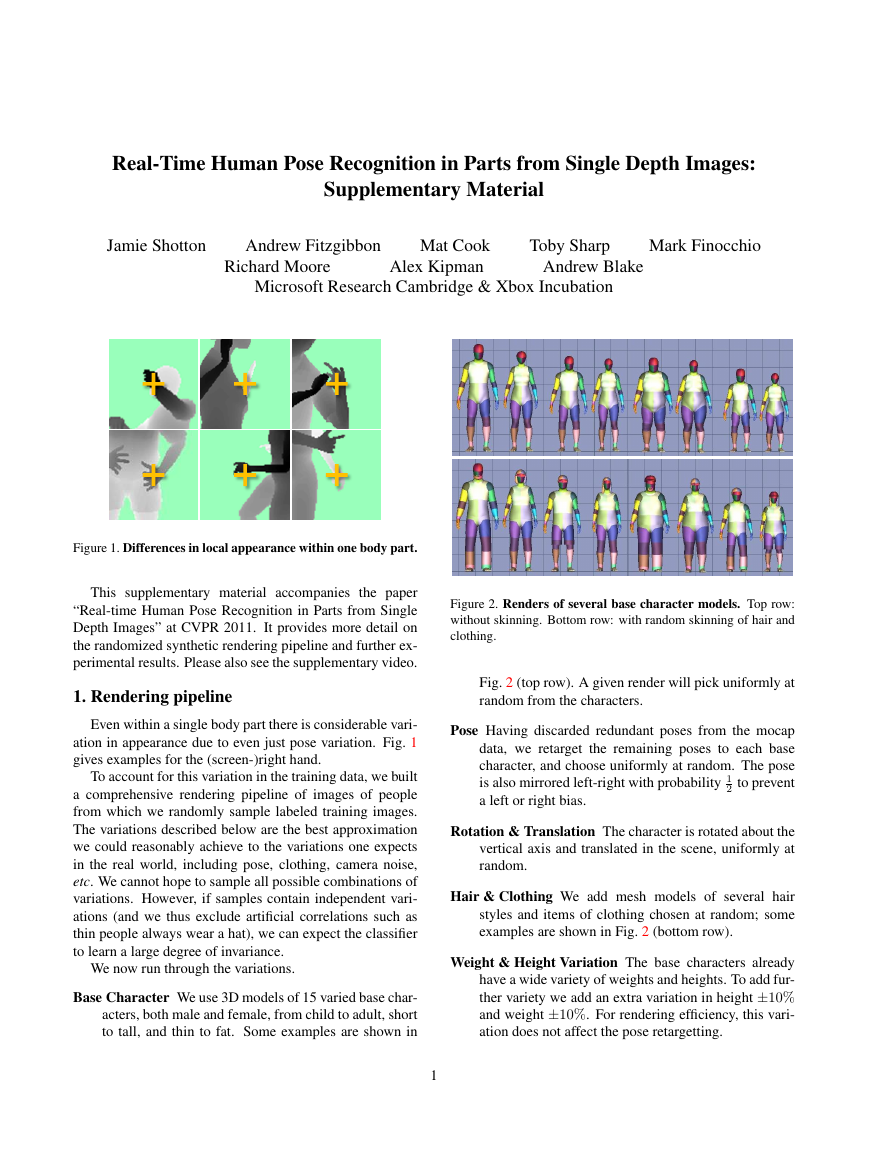
Real-Time Human Pose Recognition in Parts from Single Depth Images: Supplementary Material Jamie Shotton Andrew Fitzgibbon Richard Moore Microsoft Research Cambridge & Xbox Incubation Mat Cook Alex Kipman Toby Sharp Mark Finocchio Andrew Blake Figure 1. Differences in local appearance within one body part. This supplementary material accompanies the paper “Real-time Human Pose Recognition in Parts from Single Depth Images” at CVPR 2011. It provides more detail on the randomized synthetic rendering pipeline and further ex- perimental results. Please also see the supplementary video. 1. Rendering pipeline Even within a single body part there is considerable vari- ation in appearance due to even just pose variation. Fig. 1 gives examples for the (screen-)right hand. To account for this variation in the training data, we built a comprehensive rendering pipeline of images of people from which we randomly sample labeled training images. The variations described below are the best approximation we could reasonably achieve to the variations one expects in the real world, including pose, clothing, camera noise, etc. We cannot hope to sample all possible combinations of variations. However, if samples contain independent vari- ations (and we thus exclude artiﬁcial correlations such as thin people always wear a hat), we can expect the classiﬁer to learn a large degree of invariance. We now run through the variations. Base Character We use 3D models of 15 varied base char- acters, both male and female, from child to adult, short to tall, and thin to fat. 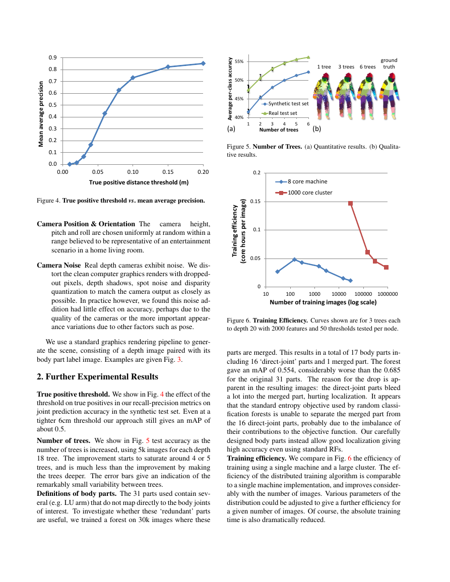Some examples are shown in 1 Figure 2. Renders of several base character models. Top row: without skinning. Bottom row: with random skinning of hair and clothing. Fig. 2 (top row). A given render will pick uniformly at random from the characters. Pose Having discarded redundant poses from the mocap data, we retarget the remaining poses to each base character, and choose uniformly at random. The pose is also mirrored left-right with probability 1 2 to prevent a left or right bias. Rotation & Translation The character is rotated about the vertical axis and translated in the scene, uniformly at random. Hair & Clothing We add mesh models of several hair styles and items of clothing chosen at random; some examples are shown in Fig. 2 (bottom row). Weight & Height Variation The base characters already have a wide variety of weights and heights. To add fur- ther variety we add an extra variation in height ±10% and weight ±10%. For rendering efﬁciency, this vari- ation does not affect the pose retargetting. Right hand appearances Base Character Models

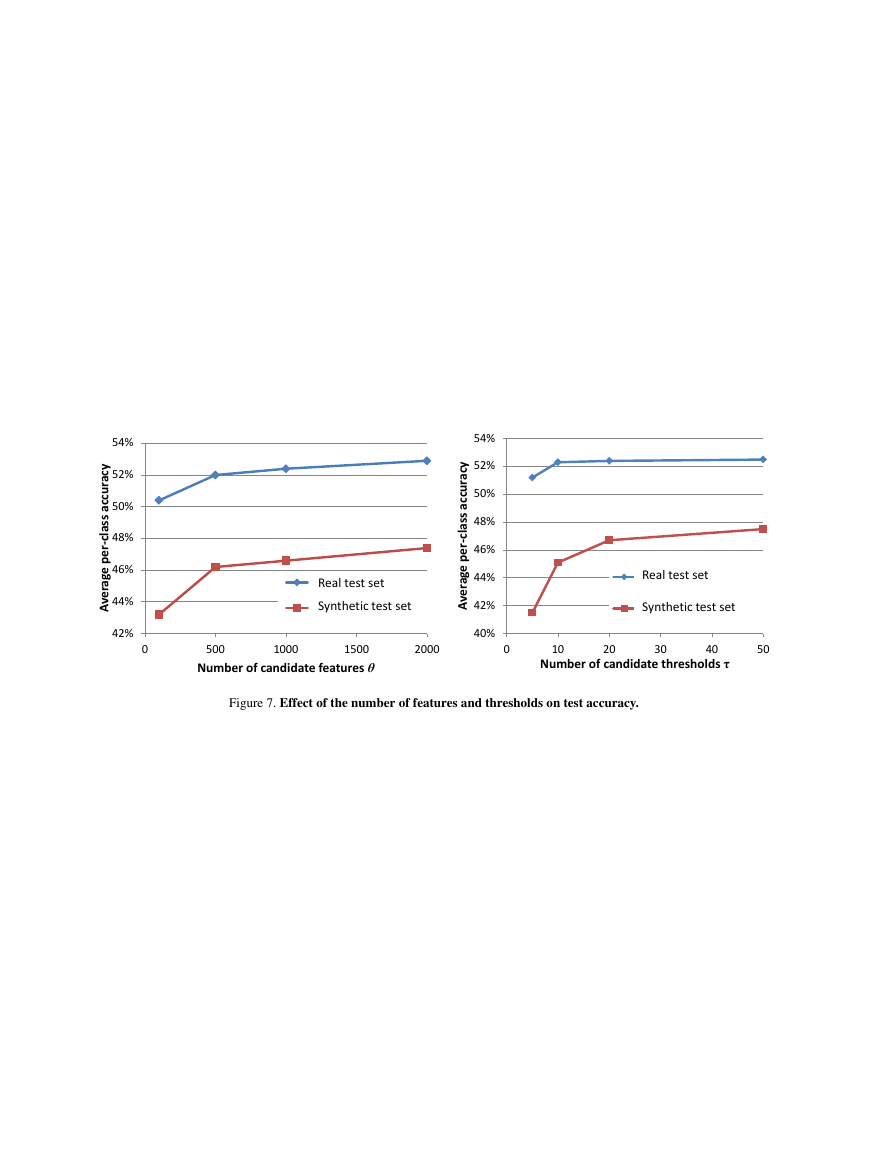
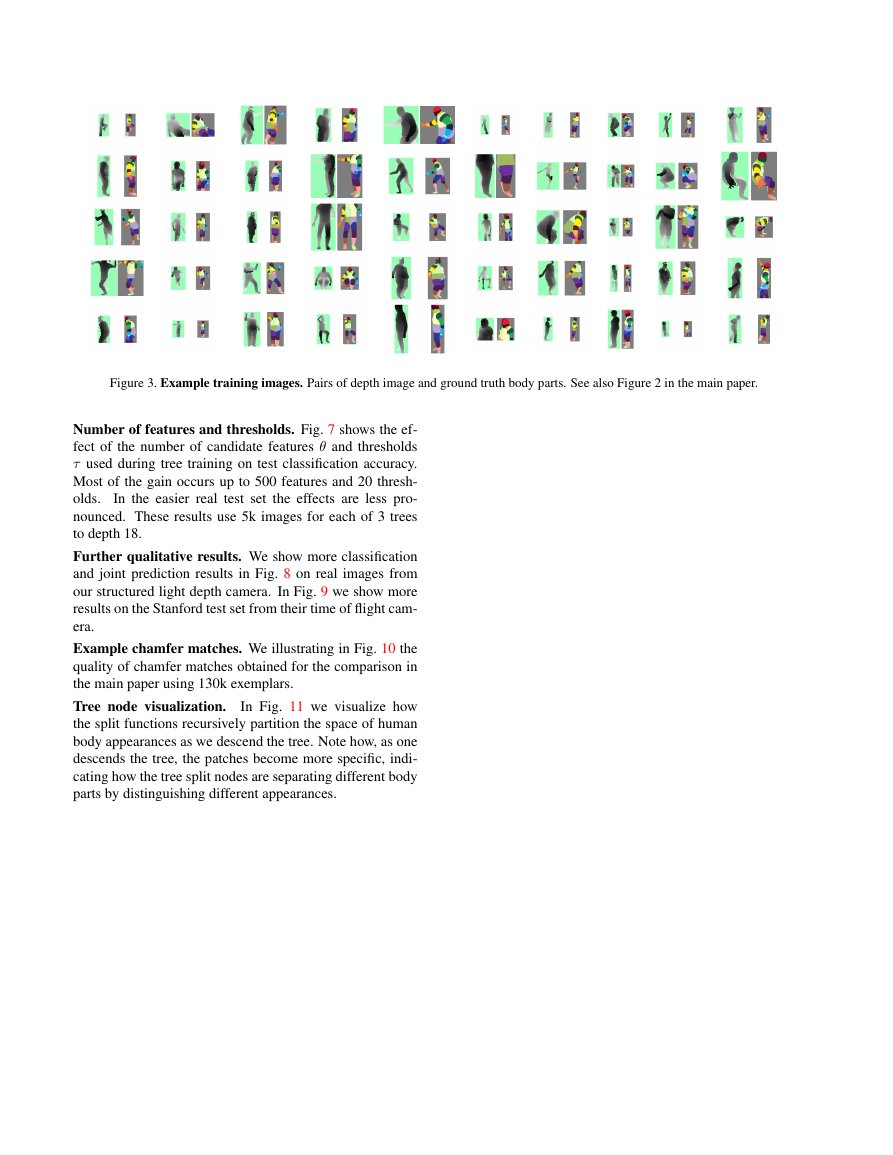
Figure 5. Number of Trees. (a) Quantitative results. (b) Qualita- tive results. Figure 4. True positive threshold vs. mean average precision. Camera Position & Orientation The height, pitch and roll are chosen uniformly at random within a range believed to be representative of an entertainment scenario in a home living room. camera Camera Noise Real depth cameras exhibit noise. We dis- tort the clean computer graphics renders with dropped- out pixels, depth shadows, spot noise and disparity quantization to match the camera output as closely as possible. In practice however, we found this noise ad- dition had little effect on accuracy, perhaps due to the quality of the cameras or the more important appear- ance variations due to other factors such as pose. We use a standard graphics rendering pipeline to gener- ate the scene, consisting of a depth image paired with its body part label image. Examples are given Fig. 3. 2. Further Experimental Results True positive threshold. We show in Fig. 4 the effect of the threshold on true positives in our recall-precision metrics on joint prediction accuracy in the synthetic test set. Even at a tighter 6cm threshold our approach still gives an mAP of about 0.5. Number of trees. We show in Fig. 5 test accuracy as the number of trees is increased, using 5k images for each depth 18 tree. The improvement starts to saturate around 4 or 5 trees, and is much less than the improvement by making the trees deeper. The error bars give an indication of the remarkably small variability between trees. Deﬁnitions of body parts. The 31 parts used contain sev- eral (e.g. LU arm) that do not map directly to the body joints of interest. To investigate whether these ‘redundant’ parts are useful, we trained a forest on 30k images where these Figure 6. Training Efﬁciency. Curves shown are for 3 trees each to depth 20 with 2000 features and 50 thresholds tested per node. parts are merged. This results in a total of 17 body parts in- cluding 16 ‘direct-joint’ parts and 1 merged part. The forest gave an mAP of 0.554, considerably worse than the 0.685 for the original 31 parts. The reason for the drop is ap- parent in the resulting images: the direct-joint parts bleed a lot into the merged part, hurting localization. It appears that the standard entropy objective used by random classi- ﬁcation forests is unable to separate the merged part from the 16 direct-joint parts, probably due to the imbalance of their contributions to the objective function. Our carefully designed body parts instead allow good localization giving high accuracy even using standard RFs. Training efﬁciency. We compare in Fig. 6 the efﬁciency of training using a single machine and a large cluster. The ef- ﬁciency of the distributed training algorithm is comparable to a single machine implementation, and improves consider- ably with the number of images. Various parameters of the distribution could be adjusted to give a further efﬁciency for a given number of images. Of course, the absolute training time is also dramatically reduced. Effect true positive threshold 0.00.10.20.30.40.50.60.70.80.90.000.050.100.150.20Mean average precision True positive distance threshold (m) 40%45%50%55%123456Average per-class accuracy Number of trees Synthetic test setReal test setNumber of trees 1 tree 3 trees 6 trees ground truth 2 tree 4 trees 5 trees (a) (b) 00.050.10.150.2101001000100001000001000000Training efficiency (core hours per image) Number of training images (log scale) 8 core machine1000 core clusterEfficiency vs Number Training Images

Figure 3. Example training images. Pairs of depth image and ground truth body parts. See also Figure 2 in the main paper. Number of features and thresholds. Fig. 7 shows the ef- fect of the number of candidate features θ and thresholds τ used during tree training on test classiﬁcation accuracy. Most of the gain occurs up to 500 features and 20 thresh- olds. In the easier real test set the effects are less pro- nounced. These results use 5k images for each of 3 trees to depth 18. 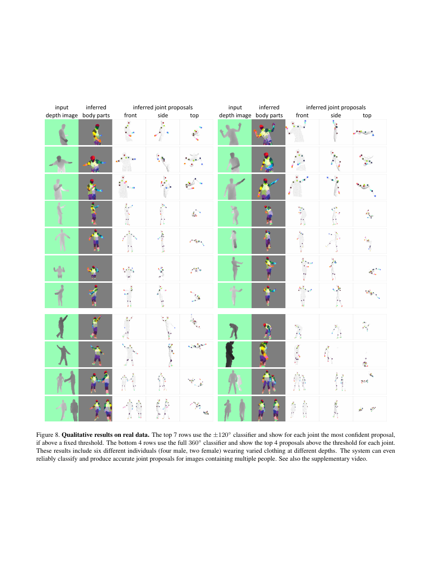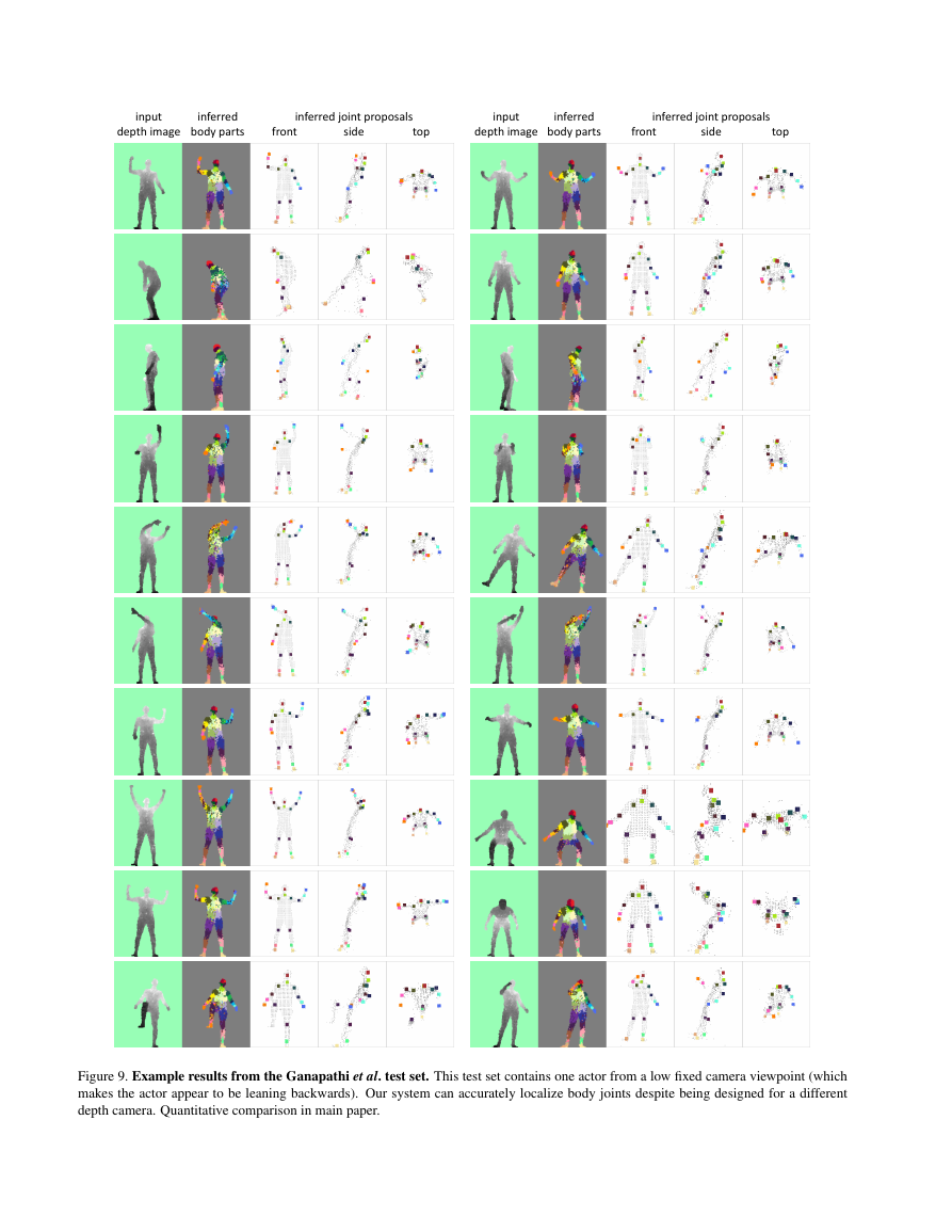Further qualitative results. We show more classiﬁcation and joint prediction results in Fig. 8 on real images from our structured light depth camera. In Fig. 9 we show more results on the Stanford test set from their time of ﬂight cam- era. 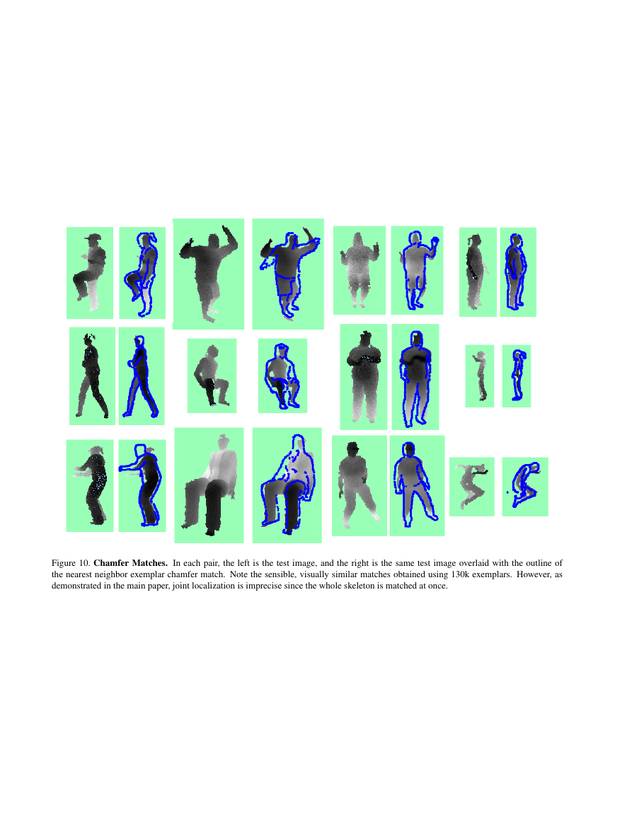Example chamfer matches. We illustrating in Fig. 10 the quality of chamfer matches obtained for the comparison in the main paper using 130k exemplars. 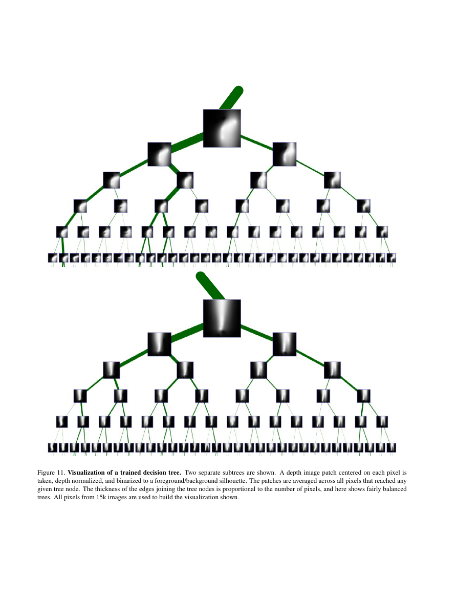Tree node visualization. In Fig. 11 we visualize how the split functions recursively partition the space of human body appearances as we descend the tree. Note how, as one descends the tree, the patches become more speciﬁc, indi- cating how the tree split nodes are separating different body parts by distinguishing different appearances. Example training images

Figure 7. Effect of the number of features and thresholds on test accuracy. Number of Features/Thresholds 42%44%46%48%50%52%54%0500100015002000Average per-class accuracy Number of candidate features θ Real test data; Uniformprobe proposalsSynthetic test data;Uniform probe proposals40%42%44%46%48%50%52%54%01020304050Average per-class accuracy Number of candidate thresholds τ Real test data; Uniformthresh. proposalsSynthetic test data;Uniform thresh. proposalsReal test set Synthetic test set Real test set Synthetic test set

Figure 8. Qualitative results on real data. The top 7 rows use the ±120◦ classiﬁer and show for each joint the most conﬁdent proposal, if above a ﬁxed threshold. The bottom 4 rows use the full 360◦ classiﬁer and show the top 4 proposals above the threshold for each joint. These results include six different individuals (four male, two female) wearing varied clothing at different depths. The system can even reliably classify and produce accurate joint proposals for images containing multiple people. See also the supplementary video. front side top input depth image inferred body parts front side top input depth image inferred body parts Example sequence results s1: 15, 160, 288, 382, 414, 436, 493, 544, 629 s2: 63, 81, 153, 173, 236, 265, 326 s3: 52, 60, 75, 92, 107, 243 s4 t1: 159, s4 t2: 192, 319, 449 s5 t1: 72, 156, 212, s5 t2: 126 inferred joint proposals inferred joint proposals

Figure 9. Example results from the Ganapathi et al. test set. This test set contains one actor from a low ﬁxed camera viewpoint (which makes the actor appear to be leaning backwards). Our system can accurately localize body joints despite being designed for a different depth camera. Quantitative comparison in main paper. Example Stanford results 0, 90, 190, 440, 580, 730, 1120,1290,1760,2360,2520,3170,3590,3940 4040, 5070, 5180, 6390,7850 front side top input depth image inferred body parts front side top input depth image inferred body parts inferred joint proposals inferred joint proposals

Figure 10. Chamfer Matches. In each pair, the left is the test image, and the right is the same test image overlaid with the outline of the nearest neighbor exemplar chamfer match. Note the sensible, visually similar matches obtained using 130k exemplars. However, as demonstrated in the main paper, joint localization is imprecise since the whole skeleton is matched at once. Chamfer matching

Figure 11. Visualization of a trained decision tree. Two separate subtrees are shown. A depth image patch centered on each pixel is taken, depth normalized, and binarized to a foreground/background silhouette. The patches are averaged across all pixels that reached any given tree node. The thickness of the edges joining the tree nodes is proportional to the number of pixels, and here shows fairly balanced trees. All pixels from 15k images are used to build the visualization shown. Views from particular nodes

资料库

微软kinect做动作识别原理的论文.pdf

相关推荐

开发技术

热门标签

最新资料