Deep Collaborative Filtering via Marginalized Denoising
Auto-encoder
∗
Sheng Li
Northeastern University
shengli@ece.neu.edu
Boston, MA, USA
Jaya Kawale
Adobe Research
San Jose, CA, USA
kawale@adobe.com
Yun Fu
Northeastern University
yunfu@ece.neu.edu
Boston, MA, USA
ABSTRACT
Collaborative filtering (CF) has been widely employed within rec-
ommender systems to solve many real-world problems. Learning
effective latent factors plays the most important role in collabora-
tive filtering. Traditional CF methods based upon matrix factoriza-
tion techniques learn the latent factors from the user-item ratings
and suffer from the cold start problem as well as the sparsity prob-
lem. Some improved CF methods enrich the priors on the latent
factors by incorporating side information as regularization. How-
ever, the learned latent factors may not be very effective due to the
sparse nature of the ratings and the side information. To tackle this
problem, we learn effective latent representations via deep learning.
Deep learning models have emerged as very appealing in learning
effective representations in many applications.
In particular, we
propose a general deep architecture for CF by integrating matrix
factorization with deep feature learning. We provide a natural in-
stantiations of our architecture by combining probabilistic matrix
factorization with marginalized denoising stacked auto-encoders.
The combined framework leads to a parsimonious fit over the latent
features as indicated by its improved performance in comparison to
prior state-of-art models over four large datasets for the tasks of
movie/book recommendation and response prediction.
Categories and Subject Descriptors
H.2.8 [Database Management]: Data Mining; H.3.3 [Information
Search Retrieval]: Information Filtering
Keywords
Collaborative filtering; matrix factorization; deep learning; denois-
ing auto-encoder
1.
INTRODUCTION
Recommendation is a fundamental problem that has gained ut-
most importance in the modern era of information overload. The
∗
Part of the work is completed during Sheng Li’s internship at
Adobe Research.
Permission to make digital or hard copies of all or part of this work for personal or
classroom use is granted without fee provided that copies are not made or distributed
for profit or commercial advantage and that copies bear this notice and the full cita-
tion on the first page. Copyrights for components of this work owned by others than
ACM must be honored. Abstracting with credit is permitted. To copy otherwise, or re-
publish, to post on servers or to redistribute to lists, requires prior specific permission
and/or a fee. Request permissions from Permissions@acm.org.
CIKM’15, October 19–23, 2015, Melbourne, Australia.
c 2015 ACM. ISBN 978-1-4503-3794-6/15/10 ...$15.00.
DOI: http://dx.doi.org/10.1145/2806416.2806527.
goal of recommendation is to help users find the item that they
maybe potentially interested in from a large repository of items.
Recommender systems are widely used by websites (e.g., Amazon,
Google News, Netflix, and Last.fm) in various contexts to target
customers and provide them with useful information. A widely
used setting of recommendation system is to predict how a user
would rate an item (such as a movie) if only given the past rating
history of the users. Many classical recommendation methods have
been proposed during the last decade. The two broad categories
of recommendation systems are content filtering approaches and
collaborative filtering (CF) based methods. The CF based meth-
ods have attracted more attention due to their impressive perfor-
mance [1]. Among various CF methods, matrix factorization has
emerged as a powerful tool to perform recommendations in large
datasets [2, 3].
Learning effective latent factors plays the most important role
in matrix factorization based CF methods. Traditional matrix fac-
torization methods for CF directly learn the latent factors from the
user-item rating matrix [2, 4]. One of the main challenges faced
by these systems is to provide a rating when a new user/item ar-
rives in the system, which is also known as the cold start scenario.
The cold start problem is circular in nature as - the system will not
recommend an item unless it has some ratings for it and unless the
system recommends it will not get ratings for it. Another practical
challenge is learning the appropriate latent factors when the rating
matrix is sparse, which is often the case in many real world scenar-
ios. In order to overcome these challenges, researchers have sug-
gested to incorporate additional sources of information about the
users or items, also known as the side information. This side infor-
mation could be obtained from the user/item profiles, for example,
demographics of a user, genre of a movie, etc. The user demo-
graphics could be used to infer the relationships between the users
and similarly the item similarity can be used to automatically as-
sign ratings to new items. The use of side information to aid matrix
factorization has been successfully applied by various prior work,
for example [5, 6, 7]. These methods, however, only utilize the side
information as regularizations in the model, and the learned latent
factors may not be very effective due to the sparse nature of the rat-
ings and the side information. In order to make matrix factorization
based methods effective in such a setting, it is highly desirable to
learn and extract discriminative features from the datasets.
One of the powerful approaches to capture feature interactions
and complex relations that has emerged in the recent past is deep
learning [8, 9]. Deep learning has attracted a lot of attention be-
cause of its promising performance to learn representations on var-
ious tasks. Deep neural networks have been shown to achieve state-
of-the-art results in computer vision, speech recognition and ma-
chine translation. The application of deep learning in recommen-
811�
dation systems, however, is very recent. With large-scale data and
rich-side information available, it is now practicable to learn latent
factors through deep architectures. Researchers have invested in
modifying deep learning algorithms like Restricted Botzmann Ma-
chines or Convolutional Neural Networks or Deep Belief Networks
directly for the task of collaborative filtering [10, 11, 12, 13, 14].
However, there are no prior work that bridge together matrix fac-
torization with deep learning methods with the notable exception
of [15]. In this paper, we present a deep learning model for collab-
orative filtering that tightly couples matrix factorization based col-
laborative filtering with deep learning algorithm namely marginal-
ized denoising auto-encoders (mDA) [16]. Unlike [15] which inte-
grates collaborative topic regression and bayesian stacked denois-
ing auto-encoders and requires learning of a large number of hy-
per parameters using an EM style algorithm, our approach uses a
much more efficient architecture based upon mDA and stochastic
gradient descent and is thus computationally efficient and highly
scalable. This paper makes the following contributions:
• We propose a general deep architecture named deep collab-
orative filtering (DCF), which integrates matrix factorization
and deep feature learning. It models the mappings between
the latent factors used in CF and the latent layers in deep
models.
• We present a practical instantiation (i.e., mDA-CF and mSDA-
CF) of the proposed architecture, by utilizing the probabilis-
tic matrix factorization and mDA. The scalability and low
computational cost of the mDA makes it a highly attractive
deep learning tool, which is unlike the prior work [15].
• We evaluate the performance of our model on three real-
world applications, movie recommendation, book recommen-
dation and response prediction. Our model outperforms con-
ventional CF methods.
2. RELATED WORK
In general, our work is closely related to the following topics:
matrix factorization based collaborative filtering, and deep learn-
ing based collaborative filtering. We will discuss the two in the
following subsections.
2.1 Matrix Factorization for Collaborative Fil-
tering
The importance of accurate recommendation techniques moti-
vated by wide ranging applications has fuelled a great amount of
academic as well as industrial research in this area [17]. Recom-
mender systems are most often based on collaborative filtering and
there are typically two approaches that are widely used. In neigh-
borhood methods, the similarity between users based on the content
they have consumed and rated is the basis of a new recommenda-
tion. A related but intrinsically more powerful approach has been
the use of latent factor models. Matrix factorization (MF) is the
most popular technique to derive latent factor models and their suc-
cess at the Netflix competition have highlighted their strength [18,
2]. For example, the given matrix X ∈ RN×M consisting of the
item preferences of the users can be decomposed as a product of
two low dimensional matrices U and V . The decomposition can
be carried out by a variety of methods ranging from SVD based
approaches [19] to the relatively new non-negative matrix factor-
ization approach [20]. One classical MF method is probabilistic
matrix factorization (PMF) [4]. The underlying assumption behind
this method is that the prior probability distribution of the latent
factors and the probability of the observed ratings given the latent
factors follows a Gaussian distribution. Many algorithms have been
developed to enhance the performance of PMF, by designing the
Bayesian versions [21, 22, 23], or incorporating side information,
such as social relationships [24, 5, 25].
Although promising, matrix factorization methods suffer from
the problem of cold-start, i.e. what recommendations to make when
a new user/item arrives in the system. Another problem often pre-
sented in many real world applications is data sparsity or reduced
coverage. Incorporating side information has shown promising per-
formance in collaborative filtering in such scenarios. Porteous et
al. proposed a Bayesian matrix factorization (BMF) approach with
side information and Dirichlet process mixtures [26]. A varia-
tional BMF method and a hierarchical BMF method that utilizes
side information were also proposed in [27] and [28], respectively.
Hu et al. proposed a cross-domain triadic factorization (CDTF)
method [29], which leverages the information from other domains.
The methods discussed above are proposed for addressing recom-
mendation problems. Recently, MF based collaborative filtering is
also applied to response prediction [30, 31]. The afore-mentioned
approaches can alleviate the problem of cold start and data sparsity
but might still suffer when the side information is sparse. Learn-
ing effective features is critical in matrix factorization. Recently,
deep learning based methods have emerged as a powerful tool for
learning representation and are widely used in many applications
ranging from computer vision to speech recognition and machine
translation.
In this paper, our goal is to combine deep learning
based methods with matrix factorization for collaborative filtering.
In the next subsection, we survey the application of deep learning
based methods for collaborative filtering.
2.2 Deep Learning for Collaborative Filtering
The application of deep learning models to the task of collabo-
rative filtering is very new and there are not much attempts in this
direction. Salakhutdinov et al. [10] were the first to apply deep
learning to the task of collaborative filtering. They modified the
restricted Boltzmann machines as a two-layer undirected graphi-
cal model consisting of binary hidden units and softmax visible
units for the task of collaborative filtering. They designed an effi-
cient learning procedure called the Contrastive Divergence (CD) to
maximize an approximation to the true likelihood function. They
also proposed a conditional RBM model and inference procedures.
They tested the performance of the model on the Netflix dataset for
movie recommendation and showed that their model performs well
as compared to the baseline methods.
Truyen et al. [14] proposed ordinal Boltzmann machines for col-
laborative filtering. They studied the parameterizations for han-
dling the ordinal nature of ratings, and presented the integration of
multiple Boltzmann machines for user-based and item-based pro-
cesses.
Recently, some deep learning models learn latent factors from
content information such as raw features of audio or articles [32,
33]. Wang et al. [12] utilized deep belief nets (DBN) for music
recommendation, which unifies feature extraction and recommen-
dation of songs in a joint framework. They assumed that a user has
a feature vector βu drawn from a Gaussian prior and the songs have
a feature vector xv. They automatically learned the feature vec-
tors of the songs using a deep belief network which is a generative
probabilistic graphical model with hidden nodes and observation.
It has millions of parameters to be learned from the training data.
The authors used stacked layers of Restricted Boltzmann Machines
for pretraining in an unsupervised fashion, and then employed the
Maximum Likelihood Estimation (MLE) for supervised learning.
812�
Oord et al. [13] addressed the music recommendation problem
using the convolutional neural networks. They first conducted a
weighted matrix factorization to handle implicit feedback and ob-
tained latent factors for all songs. After that they used deep learning
to map audio content to those latent factors. In particular, they ex-
tracted local features from audio signals and aggregated them into
a bag-of-words representation. Finally, the deep convolutional net-
work was employed to map this feature representation to the latent
factors. They tested their algorithm on the Million song dataset
and showed that their model improved the recommendation perfor-
mance by augmenting the audio signals.
All the previously mentioned approaches mainly modify the deep
learning algorithms for the task of collaborative filtering and do
not directly couple matrix factorization with deep learning models.
Most recently, Wang et al. [15] proposed a hierarchical Bayesian
model called collaborative deep learning (CDL) which tightly cou-
ples stacked denoising auto-encoders (SDA) and collaborative topic
regression (CTR). This work is the closest to our work but differs
from ours in many significant ways as follows - (i) CDL utilized
a Bayesian formulation of SDA. The generative process of CDL
consists of drawing samples for CDL uses an EM-style algorithm
for obtaining the MAP estimates of Bayesian SDA, and thus it has
to learn a large number of parameters. Our model employs a more
efficient architecture, marginalized SDA (mSDA), which computes
the parameters in closed form and is thus highly efficient and scal-
able. (ii) CDL only extracts deep features for items, whereas our
model learns deep features for both items and users.
3. PRELIMINARIES
Before we describe our general framework, we discuss the pre-
liminaries as follows.
3.1 Matrix Factorization
Matrix Factorization (MF) is the most effective collaborative fil-
tering approach. It allows us to discover the latent factors of user-
item interactions by factorizing the interactions matrix into a joint
latent space of user and item features respectively.
It proceeds
by decomposing the original rating matrix R ∈ Rm×n consist-
ing of ratings by m users for n items into two low-rank matrices
U ∈ Rm×d and V ∈ Rn×d consisting of the user and item features
respectively of rank d.
The system learns the latent factors by minimizing the following
objective function -
l(R, U, V ) +β (U2
F + V 2
F),
arg min
U,V
(1)
where l(R, U, V ) is the loss function of predicting rating using the
latent factors U and V and the last two terms are the regularizations
used to avoid overfitting. · F denotes the Frobenius norm.
Many MF-based methods have been proposed, by designing a
sophisticated loss function l(R, U, V ). Existing works usually pose
some assumptions on the latent factors U and V in (1). Probabilis-
tic matrix factorization (PMF) [4] provides a probabilistic founda-
tion by assuming a probabilistic linear model with Gaussian obser-
vation noise and Gaussian priors on the latent factors.
M
N
i=1
j=1
p(R|U, V, σ2) =
M
N (Ui|0, σ2
i Vj, σ2)Iij
N (Rij|U T
N
(2)
(3)
p(U|σ2
u) =
u) ; p(V |σ2
v) =
N (Vj|0, σ2
v).
i=1
j=1
The model is fitted by finding a MAP estimate of the parameters.
Maximizing the log posterior leads to the following objective func-
tion that can be solved using stochastic gradient descent (SGD):
arg minU,V E = R − U V
2
F + β(U2
F + V 2
F).
To improve the recommendation performance of PMF, Bayesian
probabilistic matrix factorization method (BPMF) [34] considers
a full Bayesian treatment of the parameter space instead of a point
estimate used in PMF. In the weighted matrix factorization (WMF),
)2
l(R, U, V ) = C (R − U V
F, where C is the weight ma-
trix [35]. Our model is based upon the probabilistic matrix factor-
ization approach as it has shown to have a very good performance
on several datasets and at the same time is computationally more
efficient as compared to BPMF.
When side information are available, some MF methods make
use of these additional information via regression to predict the rat-
ings [28].
3.2 Marginalized Denoising Auto-encoder (mDA)
As a specific form of neural network, an autoencoder takes a
given input and maps it (encodes) to a hidden representation via
a deterministic mapping. Denoising autoencoders reconstruct the
input from a corrupted version of the data with the motivation of
learning a more robust mapping from the data. Various types of au-
toencoders have been developed in the literature and have shown
promising results in several domains
[36, 37]. Moreover, de-
noising autoencoders can be stacked to construct a deep network
also known as stacked denoising autoencoder (SDA) which allows
learning higher level representations [38]. Despite their state-of-
the-art performance, one of the main drawbacks of SDA is the high
computational cost of training, as they rely upon the iterative and
numerical optimization techniques to learn a large amount of model
parameters.
Marginalized denoising auto-encoder (mDA) [16] is a variant of
SDA that avoids the high computational cost by marginalizing out
the random feature corruption and thus has a closed-form solution
to learn model parameters. Therefore, mDA is highly scalable and
faster than SDA. It proceeds as follows:
Given a sample set X = [x1,··· , xk], mDA considers multiple
passes (e.g., c-times) of random corruptions over X to obtain X. It
then reconstructs the input with a mapping W that minimizes the
squared loss as follows:
L(W ) = 1
2ck
xi − W ˜xij2,
(4)
c
k
j=1
i=1
where ˜xij represents the jth corrupted version of the original input
xi and W represents the mapping that is expected to minimizes the
loss function.
The above objective can be rewritten in the matrix form as
L(W ) = ¯X − W X2
F,
(5)
where ¯X = [X,··· , X] is the c-times repeated version of X, and
˜X is the corresponding corrupted version. This problem is similar
to the ordinary least squares problem and has the analytical solution
−1, where S = ˜X ˜X T , Q = ¯X ˜X T When
as given by W = SQ
c → ∞ in (4), we can derive the expectations of Q and P , and
obtain the closed form solution of the mDA [16]. Further, multi-
ple mDAs can be stacked to form a deep architecture, marginalized
stacked denoising auto-encoder (mSDA). mSDA usually enhances
the performance of mDA. Most recently, a nonlinear version of
mDA is presented [39].
813�
Table 1: Summary of notations.
Notation
m
n
d
p
q
Description
Number of users
Number of items
Dimension of latent factors
Dimension of user features
Dimension of item features
Rating matrix
Latent factors of users
Latent factors of items
R ∈ Rm×n
U ∈ Rm×d
V ∈ Rn×d
X ∈ Rp×m Side information of users
Y ∈ Rq×n
Side information of items
W1 ∈ Rp×p Mapping function for X in auto-encoder
P1 ∈ Rp×d
Projection matrix for U
4. OUR APPROACH
As we noted earlier, deep learning models have been proven to be
very effective in extracting high-level representations from the raw
input data in several learning tasks. The learned features represent
high-level knowledge. In the collaborative filtering problem, we
face a similar challenge of inferring effective latent and high-level
knowledge on user preferences from the raw inputs, including the
rating matrix and related features. MF based CF methods are able
to capture the implicit relationship between the users and the items
successfully, but they suffer from the cold start and data sparsity
problems. Therefore, it is reasonable to draw strength from the
deep models to assist the collaborative filtering process.
Table 1 summarizes the symbols used in our approach. Next, we
describe a general framework that integrates matrix factorization
and deep feature learning.
4.1 Deep Collaborative Filtering (DCF): A Gen-
eral Framework
In this section, we introduce the proposed deep collaborative fil-
tering (DCF) framework which unifies the deep learning models
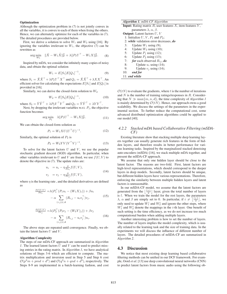
with MF based collaborative filtering. Fig. 1 illustrates the idea of
our DCF framework. DCF is a hybrid model, which makes use of
both rating matrix and side information and bridges together matrix
factorization and feature learning.
Given a user-item rating matrix R, the user side information X
and the item side information Y , DCF jointly decomposes R and
learns latent factors (i.e., U, V ) from ratings and side information
(i.e., X and Y ) through the following formulation:
arg min
U,V
l(R, U, V ) +β (U2
F + V 2
F)
+γL(X, U ) +δ L(Y, V ),
(6)
where β, γ and δ are the trade-off parameters.
There are two key components in the DCF framework: (i) the
function l(R, U, V ) for decomposing the rating matrix R into the
two latent matrices; (ii) the functions L(X, U ) and L(Y, V ) that
connect the user/item contextual features with the latent factors.
The first component derived through matrix factorization extracts
latent knowledge from the rating matrix. The second component
devised using deep learning models establishes connections of the
side information with the latent factors.
4.2 DCF using PMF + mDA
A natural instantiation of DCF is combining probabilistic matrix
factorization (PMF) with marginalized denoising auto-encoders (mDA).
PMF is a widely applied CF approach with excellent performance,
and mDA is a powerful tool in extracting high-level features from
Input layer Hidden layer Output layer
User--Item
Rating matrix
User
Feature
Feature
Item
Input layer Hidden layer Output layer
Figure 1: Illustration of DCF framework. The inputs are user-
item rating matrix R, the user feature set X and the item fea-
ture set Y . Our approach jointly decomposes R and learns la-
tent factors (i.e., U, V ) from ratings and side information (i.e.,
X and Y ). In particular, the latent factors are extracted from
the hidden layer of deep networks.
raw inputs. The combination of the two leverages their benefits for
learning even richer models.
4.2.1 mDA based Collaborative Filtering (mDA-CF)
Let ¯X ∈ Rp×cm and ¯Y ∈ Rq×cn denote the c-times repeated
versions of X and Y respectively and let ˜X and ˜Y denote their
corrupted versions. As discussed before, we utilize the loss func-
tion of PMF to decompose rating matrix R, i.e., l(R, U, V ) =
)2
A (R − U V
F, where A is the indicator matrix indicating
the non-empty entries in R and denotes the Hadamard or point-
wise product. The objective function of mDA-CF is formulated as
follows:
LU (W1, P1, U ) +L V (W2, P2, V )+
αA (R − U V
)2
F + β(U2
F + V 2
F),
(7)
arg min
U,V,W1,
W2,P1,P2
where
LU (W1, P1, U ) = ¯X − W1 ˜X2
LV (W2, P2, V ) = ¯Y − W2 ˜Y 2
F + λP1U
F + λP2V
− W1X2
F,
− W2Y 2
F,
W1 ∈ Rp×p and W2 ∈ Rq×q are reconstructive mappings, P1 ∈
Rp×d and P2 ∈ Rq×d are projection matrices, α, β and λ are trade-
off parameters. Note that, we set γ and δ in (6) to 1 for simplicity.
The first term in LU (W1, P1, U ) denotes the learning process in
marginalized denoising auto-encoder. It measures the reconstruc-
tion error between input user features ¯X and the mapped features of
corrupted inputs, i.e., W1 ˜X. W1 is the learned mapping that is ex-
pected to minimize the loss. The second term connects the hidden
layer feature W1X and the latent factor U. Generally, the latent
factor has much lower dimension than the raw features. Therefore,
we add a low-dimensional projection P1 that maps latent factor to
the feature space.
814�
Optimization
Although the optimization problem in (7) is not jointly convex in
all the variables, it is convex to each of them when fixing the others.
Hence, we can alternately optimize for each of the variables in (7).
The detailed procedures are provided below.
First, we derive a solution to solve W1 and W2 using [16]. By
ignoring the variables irrelevant to W1, the objective (7) can be
rewritten as
¯X − W1 ˜X2
F + λP1U
− W1X2
F.
(8)
arg min
W1
Inspired by mDA, we consider the infinitely many copies of noisy
data, and obtain the optimal solution
W1 = E[S1]E[Q1]
−1,
(9)
where S1 = ¯X ˜X
. An
efficient solver for calculating the expectations E[S1] and E[Q1] is
provided in [16].
and Q1 = ¯X ˜X
+ λP1U
+ λXX
X
Similarly, we can derive the closed-form solution to W2
W2 = E[S2]E[Q2]
−1,
where S2 = ¯Y ˜Y
+ λP2V
Y
and Q2 = ¯Y ˜Y
+ λY Y
.
Next, by dropping the irrelevant variables w.r.t. P1, the objective
function becomes
λP1U
− W1X2
F.
arg min
P1
We can obtain the closed-form solution as
P1 = W1XU (U
−1.
U )
Similarly, the optimal solution of P2 is
P2 = W2Y V (V
−1.
V )
To solve for the latent factors U and V , we use the popular
stochastic gradient descent (SGD) algorithm. In particular, when
other variables irrelevant to U and V are fixed, we use f (U, V ) to
denote the objective in (7). The update rules are:
ui = ui − η ∂
vj = vj − η ∂
∂ui
∂vj
f (U, V ),
f (U, V ),
(14)
where η is the learning rate , and the detailed derivatives are defined
as
∂f (U,V )
∂ui
∂f (U,V )
∂vj
1 (P1ui − (W1X)i)) + βui
=λ(P
− α
(Ri,j − uiv
j )vj.
(i,j)∈A
2 (P2vj − (W2Y )j)) + βvj
=λ(P
− α
(Ri,j − uiv
j )ui.
(i,j)∈A
The above steps are repeated until convergence. Finally, we ob-
tain the latent factors U and V .
Algorithm Complexity
The steps of our mDA-CF approach are summarized in Algorithm
1. The learned latent factors U and V can be used to predict miss-
ing entries in the rating matrix. In Algorithm 1, we have analytical
solutions of Steps 3-6 which are efficient to compute. The ma-
trix multiplication and inversion used in Step 5 and Step 6 cost
O(p2m + pmd + d3) and O(q2n + qnd + d3), respectively. The
Steps 8-9 are implemented in a batch-learning fashion, and cost
Algorithm 1. mDA-CF Algorithm
Input: Rating matrix R, user features X, item features Y ,
parameters λ, α, β.
Output: Latent factors U, V
1: Initialize U, V , P1 and P2;
2: while validation error decreases, do
3:
4:
5:
6:
7:
8:
9:
end for
10:
11: end while
Update W1 using (9);
Update W2 using (10);
Update P1 using (12);
Update P2 using (13);
for each observed Rij, do
Update ui using (14);
Update vj using (14);
O(tN ) to evaluate the gradients, where t is the number of iterations
and N is the number of training ratings/responses in R. Consider-
ing that N max{m, n, d}, the time complexity of Algorithm 1
is mainly determined by O(tN ). Hence, our approach owns a good
scalability. We discuss the settings of the parameters in the exper-
imental section. To further reduce the computational cost, some
advanced distributed optimization algorithms could be applied to
our model [40].
4.2.2
Stacked mDA based Collaborative Filtering (mSDA-
CF)
Existing literature show that stacking multiple deep learning lay-
ers together can usually generate rich features in the form of hid-
den layers, and therefore results in better performance for vari-
ous learning tasks. Inspired by the marginalized stacked denoising
auto-encoders (mSDA) [16], we stack multiple mDA together, and
present the mSDA-CF approach.
We assume that only one hidden layer should be close to the
latent factor. The reasons are two-fold. First, latent factors are
high-level representations, which should correspond to the deeper
layers in deep models. Secondly, latent factors should be unique,
but different hidden layers have various representations. Therefore,
enforcing the similarity between multiple hidden layers and latent
factors is unreasonable.
l+1
In our mSDA-CF model, we assume that the latent factors are
layer, given the total number of layers
generated from the
is l. When we train the model for the rest layers, the parameters
λ, α and β are simply set to 0. In particular, if i =
, we
only need to update W i
2 and ignore the other steps, where
W i
2 denote the mappings in the i-th layer. One benefit of
such setting is the time efficiency, as we do not increase too much
computational burden when adding multiple layers.
1 and W i
1 and W i
l+1
Another interesting problem is how to set the number of layers.
The number of layers implies the model complexity, which is usu-
ally related to the learning task and the size of training data. In the
experiments we will discuss the influence of different number of
layers. The detailed procedures of mSDA-CF are summarized in
Algorithm 2.
2
2
4.3 Discussion
We notice that most existing deep learning based collaborative
filtering methods can be unified in our DCF framework. For exam-
ple, Oord et al. [13] use deep convolutional neural networks (CNN)
to predict latent factors from music audio using the following ob-
(10)
(11)
(12)
(13)
(15)
(16)
815�
Algorithm 2. mSDA-CF Algorithm
Input: Rating matrix R, user features X, item features Y
λ, α, β, layers l.
Output: Latent factors U, V
1: for i 1 :l , do
l+1
2:
3:
if i =
, do
2
Update U and V using Algorithm 1, by setting
valid values to λ, α and β;
Update W i
λ = 0, α = 0 and β = 0;
1 and W i
2 using Algorithm 1, by setting
otherwise
4:
5:
end if
6:
7: end for
jective function:
u,i
min
θ
cu,i(pu,i − x
u y
i)2,
(17)
where xu, the latent factor of user, is estimated from weighted ma-
i, the latent factors of audio, are
trix factorization beforehand, and y
i = CNN(fv, Ω). Here, fv denotes audio
learned from CNN, i.e., y
contents, and Ω denotes the model parameters in CNN. Eqn (17)
can be interpreted in our DCF formulation (i.e., Eqn (6)). First, it
utilizes the weighted matrix factorization as the loss function l(·).
Secondly, the regularization function L(Y, V ) is implemented by
CNN.
Wang et al. [12] utilize deep belief networks (DBN) to build a
hybrid model for collaborative filtering. The objective function is
(ruv − β
uxv − r
+λγγ2
F + λyy2
F.
uyv)2 + λββ − μ2
F
(18)
u,v∈I
LHybrid =
where xv, the latent factor of item, is obtained from DBN, i.e.,
xv = DBN(fv, Ω).
Also, we can interpret model (18) in our DCF framework. First,
loss function l(·) is implemented in a hybrid way, i.e., rating ruv
is predicted by the sum of the CF part r
uyv and the content part
uxv. Secondly, DBN is employed to map the content features fv
β
and latent factor xv, which can be formulated by L(Y, V ) in DCF
framework. Meanwhile, γ in (6) is set to 0.
L = −
Wang et al. [15] propose a model with Bayesian stacked denois-
ing auto-encoders (SDAE) and collaborative topic regression are
integrated. The objective function is
2 (rij − u
i vj)2 − λn
vj − fe(X0,j∗, W +)
fr(X0,j∗, W +) − Xc,j∗2
2 − freg,
2
− λv
cij
i,j
2
2
j
2
j
(19)
where fe(·) and fr(·) denote the encoding and decoding functions
in SDAE, λn and λv denote the trade-off parameters, and freg de-
note the regularization terms that prevent overfitting.
Obviously, the model (19) can also be interpreted in the DCF
framework. The loss function for decomposing rating matrix in
(19) is in the standard matrix factorization fashion. Further, the
second and the third terms in (19) infer the item latent factor using
SDAE, which can be abstracted as L(Y, V ) in DCF.
In summary, the existing deep collaborative filtering methods
[13, 12, 15] can be unified in a common framework, DCF. We also
notice that the existing models only infer latent factors of items us-
ing deep models, whereas the latent factors of users are generated in
traditional ways. Compared to existing works, our DCF framework
provides a more flexible way to explore effective latent factors for
users and/or items via deep models.
5. EXPERIMENTS
We evaluate the performance of our mDA-CF and mSDA-CF
approaches on three challenging tasks that are movie recommenda-
tion, book recommendation and response prediction.
5.1 Movie Recommendation
For movie recommendation, we conduct experiments on two bench-
mark datasets MovieLens-100K and MovieLens-1M 1, which are
commonly used for evaluating collaborative filtering algorithms.
The MovieLens-100K dataset contains 100K ratings of 943 users
and 1682 movies, and the MovieLens-1M dataset consists of about
1 million ratings of 6040 users and 3706 movies. Each rating is
an integer between 1 (worst) and 5 (best). The ratings are highly
sparse. Table 2 summarizes the statistics of datasets. We extract
the features from side information of users and movies to construct
X and Y . To summarize, the user information which consists of
the user‘s age, gender and occupation were encoded into a binary
valued vector of length 28. Similarly, the item feature information
which consists of the 18 category of movie genre were encoded into
a binary valued vector of length 18. Ratings were normalized to be
zero-mean.
As our model (7) is an extension of the representative collab-
orative filtering method PMF, we mainly compare our approach
with PMF and its several variants, such as the Biased PMF [41]
and sparse covariance matrix factorization (SCMF) [23]. PMF and
Biased PMF are special cases of our approach mDA-CF. For ex-
ample, by adding zero weight to the first two terms in (7), mDA-
CF degrades to PMF. Further, since our approach takes advantage
of the side information of users and movies, we also compare our
approach with the collaborative filtering method that incorporates
side information, such as the Bayesian matrix factorization with
side information (BMFSI) [26].
We employ the root mean squared error (RMSE) as the evalua-
tion metric. RMSE is defined as:
ij (Rij − ˆRij)2,
Z P
(20)
i,j
RMSE =
1
N
where Rij is the ground-truth rating of user i for item j, ¯Rij de-
notes the corresponding predicted rating, N is the total number of
ratings in the test set, and Z P
ij is a binary matrix that indicates test
ratings.
For all the compared methods, we set the regularization param-
eters (e.g., λ, α and β) via 5-fold cross validation. Following the
experimental settings in [23], we train each compared method with
different percentages (50%, 80%, and 99%) of ratings. The train-
ing data are randomly chosen from each dataset, and the remaining
data are used for testing. This process is repeated five times, and
we report the average RMSE.
For the MovieLens-100K dataset, the parameters α, β and λ are
set to 0.7, 0.004 and 0.2, respectively. The learning rate used in
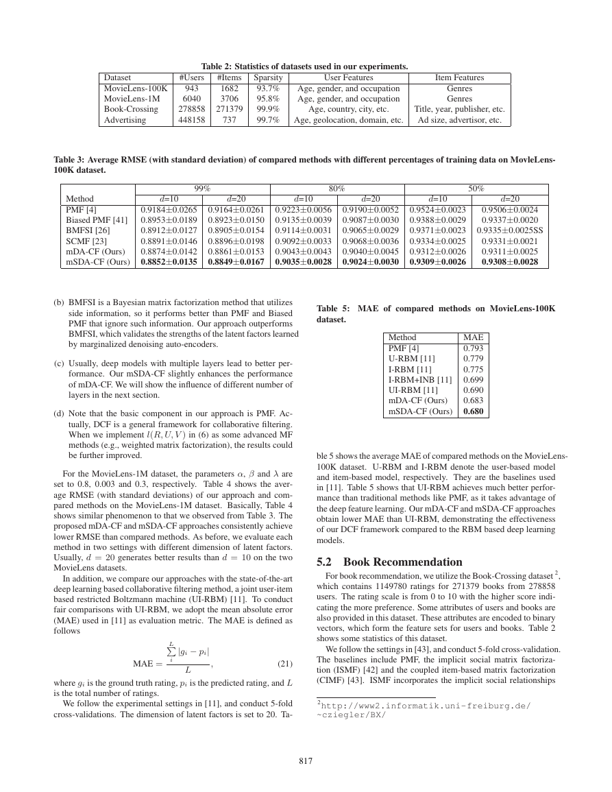
SGD is set to 0.002. Table 3 shows the average RMSE (with stan-
dard deviations) of baselines PMF, Biased PMF, BMFSI, SCMF
and our approaches, mDA-CF and mSDA-CF, on the MovieLens-
100K dataset. For each method, we have two settings for the di-
mensions of latent factors, including d = 10 and d = 20. We can
observe from Table 3 that
(a) Our approaches (mDA-CF and mSDA-CF) achieve much bet-
ter performance than PMF and Biased PMF, which are special
cases of our approach. It demonstrates the effectiveness of in-
corporating side information and deep architectures.
1http://grouplens.org/datasets/movielens/
816�
Table 2: Statistics of datasets used in our experiments.
Dataset
MovieLens-100K
MovieLens-1M
Book-Crossing
Advertising
#Users
943
6040
278858
448158
#Items
1682
3706
271379
737
User Features
Sparsity
93.7%
95.8%
99.9%
99.7% Age, geolocation, domain, etc.
Age, gender, and occupation
Age, gender, and occupation
Age, country, city, etc.
Item Features
Genres
Genres
Title, year, publisher, etc.
Ad size, advertisor, etc.
Table 3: Average RMSE (with standard deviation) of compared methods with different percentages of training data on MovleLens-
100K dataset.
99%
80%
Method
PMF [4]
Biased PMF [41]
BMFSI [26]
SCMF [23]
mDA-CF (Ours)
mSDA-CF (Ours)
d=10
0.9184±0.0265
0.8953±0.0189
0.8912±0.0127
0.8891±0.0146
0.8874±0.0142
0.8852±0.0135
d=20
0.9164±0.0261
0.8923±0.0150
0.8905±0.0154
0.8896±0.0198
0.8861±0.0153
0.8849±0.0167
d=10
0.9223±0.0056
0.9135±0.0039
0.9114±0.0031
0.9092±0.0033
0.9043±0.0043
0.9035±0.0028
d=20
0.9190±0.0052
0.9087±0.0030
0.9065±0.0029
0.9068±0.0036
0.9040±0.0045
0.9024±0.0030
d=10
0.9524±0.0023
0.9388±0.0029
0.9371±0.0023
0.9334±0.0025
0.9312±0.0026
0.9309±0.0026
50%
d=20
0.9506±0.0024
0.9337±0.0020
0.9335±0.0025SS
0.9331±0.0021
0.9311±0.0025
0.9308±0.0028
(b) BMFSI is a Bayesian matrix factorization method that utilizes
side information, so it performs better than PMF and Biased
PMF that ignore such information. Our approach outperforms
BMFSI, which validates the strengths of the latent factors learned
by marginalized denoising auto-encoders.
(c) Usually, deep models with multiple layers lead to better per-
formance. Our mSDA-CF slightly enhances the performance
of mDA-CF. We will show the influence of different number of
layers in the next section.
(d) Note that the basic component in our approach is PMF. Ac-
tually, DCF is a general framework for collaborative filtering.
When we implement l(R, U, V ) in (6) as some advanced MF
methods (e.g., weighted matrix factorization), the results could
be further improved.
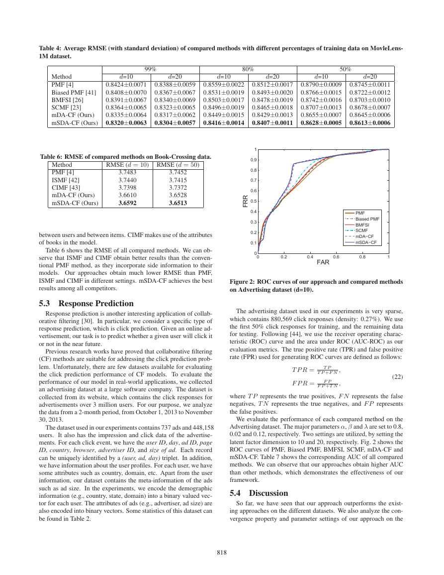
For the MovieLens-1M dataset, the parameters α, β and λ are
set to 0.8, 0.003 and 0.3, respectively. Table 4 shows the aver-
age RMSE (with standard deviations) of our approach and com-
pared methods on the MovieLens-1M dataset. Basically, Table 4
shows similar phenomenon to that we observed from Table 3. The
proposed mDA-CF and mSDA-CF approaches consistently achieve
lower RMSE than compared methods. As before, we evaluate each
method in two settings with different dimension of latent factors.
Usually, d = 20 generates better results than d = 10 on the two
MovieLens datasets.
In addition, we compare our approaches with the state-of-the-art
deep learning based collaborative filtering method, a joint user-item
based restricted Boltzmann machine (UI-RBM) [11]. To conduct
fair comparisons with UI-RBM, we adopt the mean absolute error
(MAE) used in [11] as evaluation metric. The MAE is defined as
follows
L
MAE =
i
|gi − pi|
,
L
(21)
where gi is the ground truth rating, pi is the predicted rating, and L
is the total number of ratings.
We follow the experimental settings in [11], and conduct 5-fold
cross-validations. The dimension of latent factors is set to 20. Ta-
Table 5: MAE of compared methods on MovieLens-100K
dataset.
Method
PMF [4]
U-RBM [11]
I-RBM [11]
I-RBM+INB [11]
UI-RBM [11]
mDA-CF (Ours)
mSDA-CF (Ours)
MAE
0.793
0.779
0.775
0.699
0.690
0.683
0.680
ble 5 shows the average MAE of compared methods on the MovieLens-
100K dataset. U-RBM and I-RBM denote the user-based model
and item-based model, respectively. They are the baselines used
in [11]. Table 5 shows that UI-RBM achieves much better perfor-
mance than traditional methods like PMF, as it takes advantage of
the deep feature learning. Our mDA-CF and mSDA-CF approaches
obtain lower MAE than UI-RBM, demonstrating the effectiveness
of our DCF framework compared to the RBM based deep learning
models.
5.2 Book Recommendation
For book recommendation, we utilize the Book-Crossing dataset 2,
which contains 1149780 ratings for 271379 books from 278858
users. The rating scale is from 0 to 10 with the higher score indi-
cating the more preference. Some attributes of users and books are
also provided in this dataset. These attributes are encoded to binary
vectors, which form the feature sets for users and books. Table 2
shows some statistics of this dataset.
We follow the settings in [43], and conduct 5-fold cross-validation.
The baselines include PMF, the implicit social matrix factoriza-
tion (ISMF) [42] and the coupled item-based matrix factorization
(CIMF) [43]. ISMF incorporates the implicit social relationships
2http://www2.informatik.uni-freiburg.de/
~cziegler/BX/
817�
Table 4: Average RMSE (with standard deviation) of compared methods with different percentages of training data on MovleLens-
1M dataset.
99%
Method
PMF [4]
Biased PMF [41]
BMFSI [26]
SCMF [23]
mDA-CF (Ours)
mSDA-CF (Ours)
d=10
0.8424±0.0071
0.8408±0.0070
0.8391±0.0067
0.8364±0.0065
0.8335±0.0064
0.8320±0.0063
d=20
0.8388±0.0059
0.8367±0.0067
0.8340±0.0069
0.8323±0.0065
0.8317±0.0062
0.8304±0.0057
80%
50%
d=10
0.8559±0.0022
0.8531±0.0019
0.8503±0.0017
0.8496±0.0019
0.8449±0.0015
0.8416±0.0014
d=20
0.8512±0.0017
0.8493±0.0020
0.8478±0.0019
0.8465±0.0018
0.8429±0.0013
0.8407±0.0011
d=10
0.8790±0.0009
0.8766±0.0015
0.8742±0.0016
0.8707±0.0013
0.8655±0.0007
0.8628±0.0005
d=20
0.8745±0.0011
0.8722±0.0012
0.8703±0.0010
0.8678±0.0007
0.8645±0.0006
0.8613±0.0006
Table 6: RMSE of compared methods on Book-Crossing data.
RMSE (d = 10) RMSE (d = 50)
Method
PMF [4]
ISMF [42]
CIMF [43]
mDA-CF (Ours)
mSDA-CF (Ours)
3.7483
3.7440
3.7398
3.6610
3.6592
3.7452
3.7415
3.7372
3.6528
3.6513
between users and between items. CIMF makes use of the attributes
of books in the model.
Table 6 shows the RMSE of all compared methods. We can ob-
serve that ISMF and CIMF obtain better results than the conven-
tional PMF method, as they incorporate side information to their
models. Our approaches obtain much lower RMSE than PMF,
ISMF and CIMF in different settings. mSDA-CF achieves the best
results among all competitors.
5.3 Response Prediction
Response prediction is another interesting application of collab-
orative filtering [30]. In particular, we consider a specific type of
response prediction, which is click prediction. Given an online ad-
vertisement, our task is to predict whether a given user will click it
or not in the near future.
Previous research works have proved that collaborative filtering
(CF) methods are suitable for addressing the click prediction prob-
lem. Unfortunately, there are few datasets available for evaluating
the click prediction performance of CF models. To evaluate the
performance of our model in real-world applications, we collected
an advertising dataset at a large software company. The dataset is
collected from its website, which contains the click responses for
advertisements over 3 million users. For our purpose, we analyze
the data from a 2-month period, from October 1, 2013 to November
30, 2013.
The dataset used in our experiments contains 737 ads and 448,158
users. It also has the impression and click data of the advertise-
ments. For each click event, we have the user ID, day, ad ID, page
ID, country, browser, advertiser ID, and size of ad. Each record
can be uniquely identified by a (user, ad, day) triplet. In addition,
we have information about the user profiles. For each user, we have
some attributes such as country, domain, etc. Apart from the user
information, our dataset contains the meta-information of the ads
such as ad size. In the experiments, we encode the demographic
information (e.g., country, state, domain) into a binary valued vec-
tor for each user. The attributes of ads (e.g., advertiser, ad size) are
also encoded into binary vectors. Some statistics of this dataset can
be found in Table 2.
1
0.9
0.8
0.7
0.6
0.5
0.4
0.3
0.2
0.1
R
R
F
PMF
Biased PMF
BMFSI
SCMF
mDA−CF
mSDA−CF
0
0
0.2
0.4
0.6
0.8
1
FAR
Figure 2: ROC curves of our approach and compared methods
on Advertising dataset (d=10).
The advertising dataset used in our experiments is very sparse,
which contains 880,569 click responses (density: 0.27%). We use
the first 50% click responses for training, and the remaining data
for testing. Following [44], we use the receiver operating charac-
teristic (ROC) curve and the area under ROC (AUC-ROC) as our
evaluation metrics. The true positive rate (TPR) and false positive
rate (FPR) used for generating ROC curves are defined as follows:
T P R = T P
T P +F N ,
F P R = F P
F P +T N ,
(22)
where T P represents the true positives, F N represents the false
negatives, T N represents the true negatives, and F P represents
the false positives.
We evaluate the performance of each compared method on the
Advertising dataset. The major parameters α, β and λ are set to 0.8,
0.02 and 0.12, respectively. Two settings are utilized, by setting the
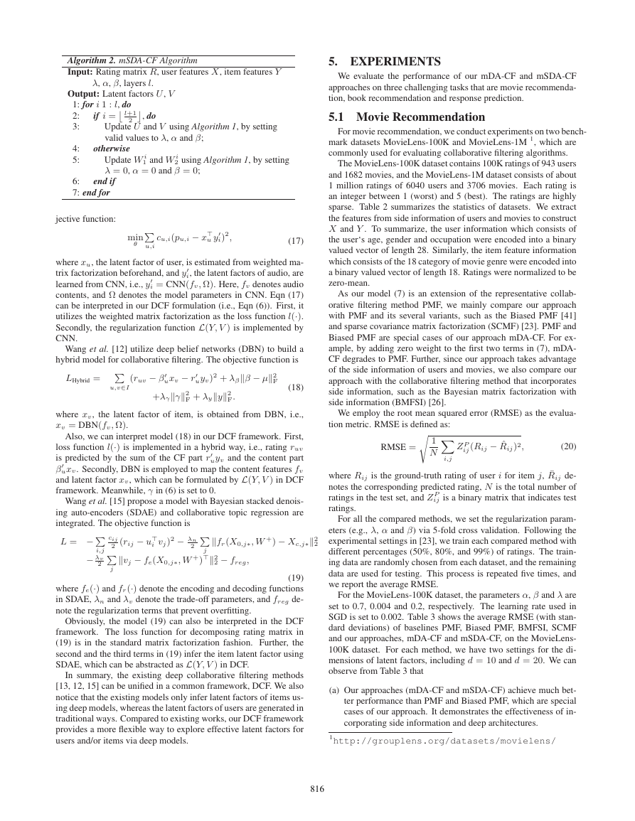
latent factor dimension to 10 and 20, respectively. Fig. 2 shows the
ROC curves of PMF, Biased PMF, BMFSI, SCMF, mDA-CF and
mSDA-CF. Table 7 shows the corresponding AUC of all compared
methods. We can observe that our approaches obtain higher AUC
than other methods, which demonstrates the effectiveness of our
framework.
5.4 Discussion
So far, we have seen that our approach outperforms the exist-
ing approaches on the different datasets. We also analyze the con-
vergence property and parameter settings of our approach on the
818�


 2023年江西萍乡中考道德与法治真题及答案.doc
 2012年重庆南川中考生物真题及答案.doc
 2013年江西师范大学地理学综合及文艺理论基础考研真题.doc
 2020年四川甘孜小升初语文真题及答案I卷.doc
 2020年注册岩土工程师专业基础考试真题及答案.doc
 2023-2024学年福建省厦门市九年级上学期数学月考试题及答案.doc
 2021-2022学年辽宁省沈阳市大东区九年级上学期语文期末试题及答案.doc
 2022-2023学年北京东城区初三第一学期物理期末试卷及答案.doc
 2018上半年江西教师资格初中地理学科知识与教学能力真题及答案.doc
 2012年河北国家公务员申论考试真题及答案-省级.doc
 2020-2021学年江苏省扬州市江都区邵樊片九年级上学期数学第一次质量检测试题及答案.doc
 2022下半年黑龙江教师资格证中学综合素质真题及答案.doc