Comparison of Multiobjective Evolutionary
Algorithms: Empirical Results
Kalyanmoy Deb
Department of Mechanical Engineering
Indian Institute of Technology Kanpur
Kanpur, PIN 208 016, India
deb@iitk.ac.in
Eckart Zitzler
Department of Electrical Engineering
Swiss Federal Institute of Technology
8092 Zurich, Switzerland
zitzler@tik.ee.ethz.ch
Lothar Thiele
Department of Electrical Engineering
Swiss Federal Institute of Technology
8092 Zurich, Switzerland
thiele@tik.ee.ethz.ch
Abstract
In this paper, we provide a systematic comparison of various evolutionary approaches to
multiobjective optimization using six carefully chosen test functions. Each test function
involves a particular feature that is known to cause difficulty in the evolutionary optimiza-
tion process, mainly in converging to the Pareto-optimal front (e.g., multimodality and
deception). By investigating these different problem features separately, it is possible to
predict the kind of problems to which a certain technique is or is not well suited. However,
in contrast to what was suspected beforehand, the experimental results indicate a hierarchy
of the algorithms under consideration. Furthermore, the emerging effects are evidence
that the suggested test functions provide sufficient complexity to compare multiobjective
optimizers. Finally, elitism is shown to be an important factor for improving evolutionary
multiobjective search.
Keywords
Evolutionary algorithms, multiobjective optimization, Pareto optimality, test functions,
elitism.
1 Motivation
Evolutionary algorithms (EAs) have become established as the method at hand for exploring
the Pareto-optimal front in multiobjective optimization problems that are too complex to
be solved by exact methods, such as linear programming and gradient search. This is not
only because there are few alternatives for searching intractably large spaces for multiple
Pareto-optimal solutions. Due to their inherent parallelism and their capability to exploit
similarities of solutions by recombination, they are able to approximate the Pareto-optimal
front in a single optimization run. The numerous applications and the rapidly growing
interest in the area of multiobjective EAs take this fact into account.
After the first pioneering studies on evolutionary multiobjective optimization appeared
in the mid-eighties (Schaffer, 1984, 1985; Fourman,1985) several different EA implementa-
tions were proposed in the years 1991–1994 (Kursawe, 1991; Hajela and Lin, 1992; Fonseca
c2000 by the Massachusetts Institute of Technology
Evolutionary Computation 8(2): 173-195
�
E. Zitzler, K. Deb, and L. Thiele
and Fleming, 1993; Horn et al., 1994; Srinivas and Deb, 1994). Later, these approaches
(and variations of them) were successfully applied to various multiobjective optimization
problems (Ishibuchi and Murata, 1996; Cunha et al., 1997; Valenzuela-Rend ´on and Uresti-
Charre, 1997; Fonseca and Fleming, 1998; Parks and Miller, 1998). In recent years, some
researchers have investigated particular topics of evolutionary multiobjective search, such
as convergence to the Pareto-optimal front (Van Veldhuizen and Lamont, 1998a; Rudolph,
1998), niching (Obayashi et al., 1998), and elitism (Parks and Miller, 1998; Obayashi et al.,
1998), while others have concentrated on developing new evolutionary techniques (Lau-
manns et al., 1998; Zitzler and Thiele, 1999). For a thorough discussion of evolutionary
algorithms for multiobjective optimization, the interested reader is referred to Fonseca and
Fleming (1995), Horn (1997), Van Veldhuizen and Lamont (1998b), and Coello (1999).
In spite of this variety, there is a lack of studies that compare the performance and
different aspects of these approaches. Consequently, the question arises: which imple-
mentations are suited to which sort of problem, and what are the specific advantages and
drawbacks of different techniques?
First steps in this direction have been made in both theory and practice. On the
theoretical side, Fonseca and Fleming (1995) discussed the influence of different fitness
assignment strategies on the selection process. On the practical side, Zitzler and Thiele
(1998, 1999) used a NP-hard 0/1 knapsack problem to compare several multiobjective EAs.
In this paper, we provide a systematic comparison of six multiobjective EAs, including a
random search strategy as well as a single-objective EA using objective aggregation. The
basis of this empirical study is formed by a set of well-defined, domain-independent test
functions that allow the investigation of independent problem features. We thereby draw
upon results presented in Deb (1999), where problem features that may make convergence
of EAs to the Pareto-optimal front difficult are identified and, furthermore, methods of
constructing appropriate test functions are suggested. The functions considered here cover
the range of convexity, nonconvexity, discrete Pareto fronts, multimodality, deception, and
biased search spaces. Hence, we are able to systematically compare the approaches based
on different kinds of difficulty and to determine more exactly where certain techniques
are advantageous or have trouble. In this context, we also examine further factors such as
population size and elitism.
The paper is structured as follows: Section 2 introduces key concepts of multiobjective
optimization and defines the terminology used in this paper mathematically. We then give
a brief overview of the multiobjective EAs under consideration with special emphasis on
the differences between them. The test functions, their construction, and their choice
are the subject of Section 4, which is followed by a discussion about performance metrics
to assess the quality of trade-off fronts. Afterwards, we present the experimental results
in Section 6 and investigate further aspects like elitism (Section 7) and population size
(Section 8) separately. A discussion of the results as well as future perspectives are given in
Section 9.
2 Definitions
Optimization problems involving multiple, conflicting objectives are often approached by
aggregating the objectives into a scalar function and solving the resulting single-objective
optimization problem. In contrast, in this study, we are concerned with finding a set of
optimal trade-offs, the so-called Pareto-optimal set. In the following, we formalize this
174
Evolutionary Computation Volume 8, Number 2
�
Comparison of Multiobjective EAs
well-known concept and also define the difference between local and global Pareto-optimal
sets.
A multiobjective search space is partially ordered in the sense that two arbitrary so-
lutions are related to each other in two possible ways: either one dominates the other or
neither dominates.
DEFINITION 1: Let us consider, without loss of generality, a multiobjective minimization problem
with m decision variables (parameters) and n objectives:
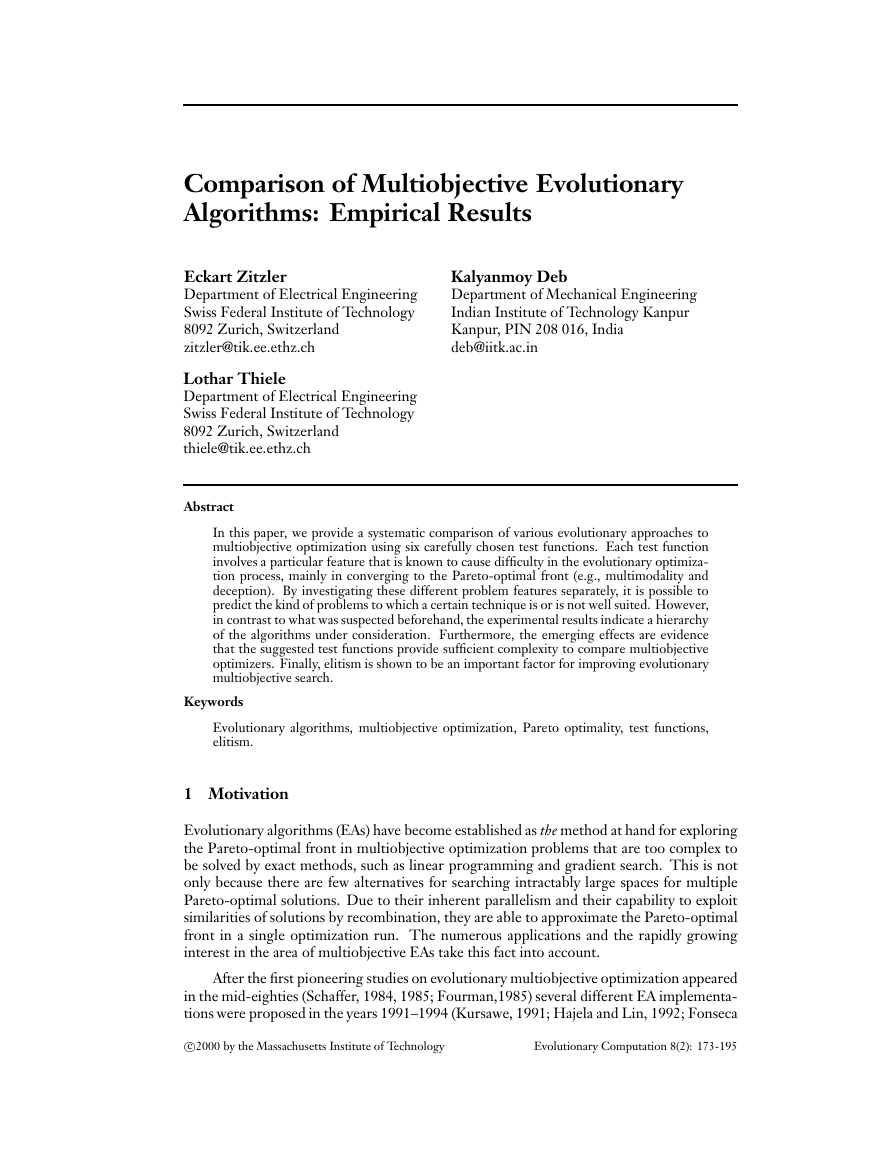
Minimize y f x f�x fnx
where
x x� xm � X
y y� yn � Y
(1)
and where x is called decision vector, X parameter space, y objective vector, and Y objective
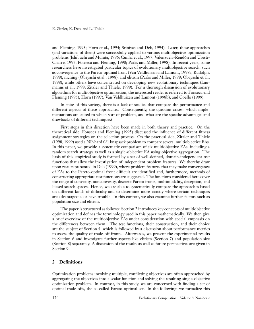
space. A decision vector a � X is said to dominate a decision vector b � X (also written as a b)
if and only if
�i � f� ng
j � f� ng
fia fib
fja fjb
(2)
Additionally, in this study, we say a covers b (a b) if and only if a b or f a f b.
Based on the above relation, we can define nondominated and Pareto-optimal solutions:
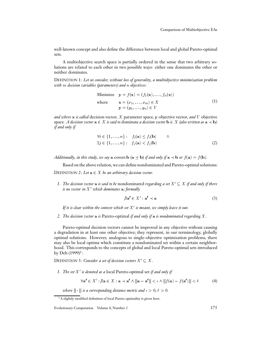
DEFINITION 2: Let a � X be an arbitrary decision vector.
1. The decision vector a is said to be nondominated regarding a set X � X if and only if there
is no vector in X � which dominates a; formally
� a� � X � a� a
(3)
If it is clear within the context which set X � is meant, we simply leave it out.
2. The decision vector a is Pareto-optimal if and only if a is nondominated regarding X.
Pareto-optimal decision vectors cannot be improved in any objective without causing
a degradation in at least one other objective; they represent, in our terminology, globally
optimal solutions. However, analogous to single-objective optimization problems, there
may also be local optima which constitute a nondominated set within a certain neighbor-
hood. This corresponds to the concepts of global and local Pareto-optimal sets introduced
by Deb (1999)�:
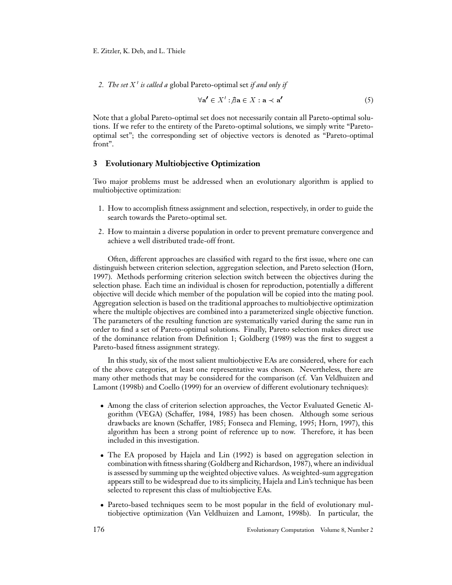
DEFINITION 3: Consider a set of decision vectors X � X.
1. The set X � is denoted as a local Pareto-optimal set if and only if
�a� � X � � a � X a a� jja a�jj jjf a f a�jj
where jj jj is a corresponding distance metric and �, �.
�A slightly modified definition of local Pareto optimality is given here.
Evolutionary Computation Volume 8, Number 2
(4)
175
�
E. Zitzler, K. Deb, and L. Thiele
2. The set X � is called a global Pareto-optimal set if and only if
�a� � X � � a � X a a�
(5)
Note that a global Pareto-optimal set does not necessarily contain all Pareto-optimal solu-
tions. If we refer to the entirety of the Pareto-optimal solutions, we simply write “Pareto-
optimal set”; the corresponding set of objective vectors is denoted as “Pareto-optimal
front”.
3 Evolutionary Multiobjective Optimization
Two major problems must be addressed when an evolutionary algorithm is applied to
multiobjective optimization:
1. How to accomplish fitness assignment and selection, respectively, in order to guide the
search towards the Pareto-optimal set.
2. How to maintain a diverse population in order to prevent premature convergence and
achieve a well distributed trade-off front.
Often, different approaches are classified with regard to the first issue, where one can
distinguish between criterion selection, aggregation selection, and Pareto selection (Horn,
1997). Methods performing criterion selection switch between the objectives during the
selection phase. Each time an individual is chosen for reproduction, potentially a different
objective will decide which member of the population will be copied into the mating pool.
Aggregation selection is based on the traditional approaches to multiobjective optimization
where the multiple objectives are combined into a parameterized single objective function.
The parameters of the resulting function are systematically varied during the same run in
order to find a set of Pareto-optimal solutions. Finally, Pareto selection makes direct use
of the dominance relation from Definition 1; Goldberg (1989) was the first to suggest a
Pareto-based fitness assignment strategy.
In this study, six of the most salient multiobjective EAs are considered, where for each
of the above categories, at least one representative was chosen. Nevertheless, there are
many other methods that may be considered for the comparison (cf. Van Veldhuizen and
Lamont (1998b) and Coello (1999) for an overview of different evolutionary techniques):
Among the class of criterion selection approaches, the Vector Evaluated Genetic Al-
gorithm (VEGA) (Schaffer, 1984, 1985) has been chosen. Although some serious
drawbacks are known (Schaffer, 1985; Fonseca and Fleming, 1995; Horn, 1997), this
algorithm has been a strong point of reference up to now. Therefore, it has been
included in this investigation.
The EA proposed by Hajela and Lin (1992) is based on aggregation selection in
combination with fitness sharing (Goldberg and Richardson, 1987), where an individual
is assessed by summing up the weighted objective values. As weighted-sum aggregation
appears still to be widespread due to its simplicity, Hajela and Lin’s technique has been
selected to represent this class of multiobjective EAs.
Pareto-based techniques seem to be most popular in the field of evolutionary mul-
In particular, the
tiobjective optimization (Van Veldhuizen and Lamont, 1998b).
176
Evolutionary Computation Volume 8, Number 2
�
Comparison of Multiobjective EAs
algorithm presented by Fonseca and Fleming (1993), the Niched Pareto Genetic Algo-
rithm (NPGA) (Horn and Nafpliotis, 1993; Horn et al., 1994), and the Nondominated
Sorting Genetic Algorithm (NSGA) (Srinivas and Deb, 1994) appear to have achieved
the most attention in the EA literature and have been used in various studies. Thus,
they are also considered here. Furthermore, a recent elitist Pareto-based strategy, the
Strength Pareto Evolutionary Algorithm (SPGA) (Zitzler and Thiele, 1999), which
outperformed four other multiobjective EAs on an extended 0/1 knapsack problem, is
included in the comparison.
4 Test Functions for Multiobjective Optimizers
Deb (1999) has identified several features that may cause difficulties for multiobjective
EAs in 1) converging to the Pareto-optimal front and 2) maintaining diversity within the
population. Concerning the first issue, multimodality, deception, and isolated optima are
well-known problem areas in single-objective evolutionary optimization. The second issue
is important in order to achieve a well distributed nondominated front. However, certain
characteristics of the Pareto-optimal front may prevent an EA from finding diverse Pareto-
optimal solutions: convexity or nonconvexity, discreteness, and nonuniformity. For each of
the six problem features mentioned, a corresponding test function is constructed following
the guidelines in Deb (1999). We thereby restrict ourselves to only two objectives in
order to investigate the simplest case first. In our opinion, two objectives are sufficient
to reflect essential aspects of multiobjective optimization. Moreover, we do not consider
maximization or mixed minimization/maximization problems.
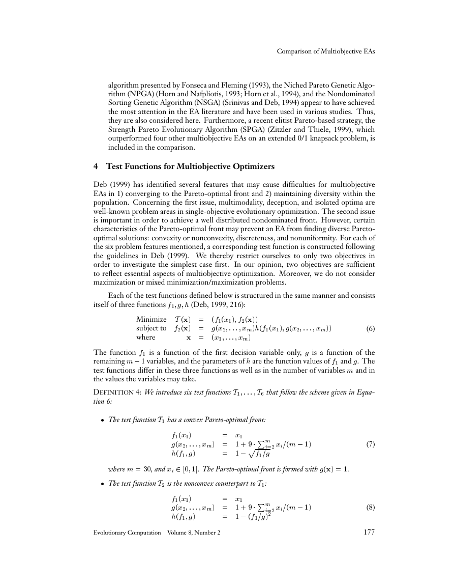
Each of the test functions defined below is structured in the same manner and consists
itself of three functions f� g h (Deb, 1999, 216):
T x f�x� f�x
Minimize
subject to f�x gx� xmhf�x� gx� xm
where
x x� xm
(6)
The function f� is a function of the first decision variable only, g is a function of the
remaining m � variables, and the parameters of h are the function values of f� and g. The
test functions differ in these three functions as well as in the number of variables m and in
the values the variables may take.
DEFINITION 4: We introduce six test functions T� T� that follow the scheme given in Equa-
tion 6:
The test function T� has a convex Pareto-optimal front:
f�x�
x�
gx� xm � Pm
� pf�g
hf� g
i� xim �
where m ��, and xi � � �. The Pareto-optimal front is formed with gx �.
The test function T� is the nonconvex counterpart to T�:
f�x�
x�
gx� xm � Pm
� f�g�
hf� g
i� xim �
Evolutionary Computation Volume 8, Number 2
(7)
(8)
177
�
E. Zitzler, K. Deb, and L. Thiele
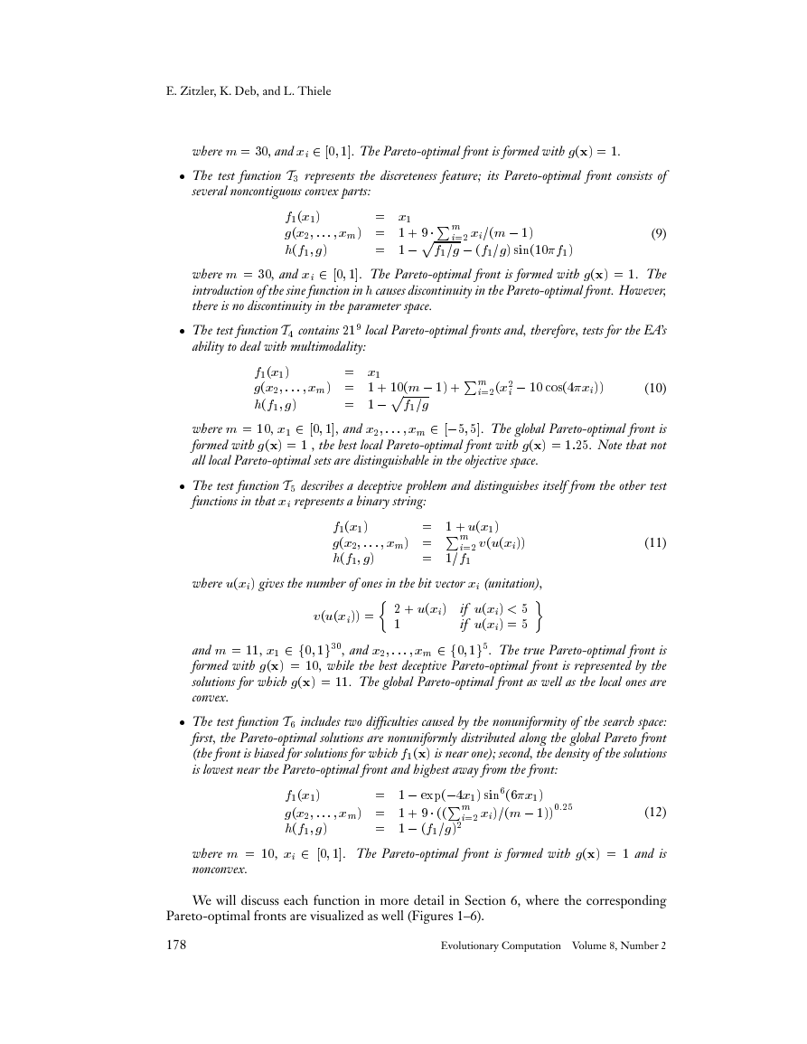
where m ��, and xi � � �. The Pareto-optimal front is formed with gx �.
The test function T� represents the discreteness feature; its Pareto-optimal front consists of
several noncontiguous convex parts:
f�x�
x�
gx� xm � Pm
hf� g
i� xim �
� pf�g f�g sin��f�
(9)
where m ��, and xi � � �. The Pareto-optimal front is formed with gx �. The
introduction of the sine function in h causes discontinuity in the Pareto-optimal front. However,
there is no discontinuity in the parameter space.
The test function T� contains �� local Pareto-optimal fronts and, therefore, tests for the EA’s
ability to deal with multimodality:
f�x�
x�
gx� xm � ��m � Pm
hf� g
� pf�g
i�x�
i �� cos�xi
(10)
where m ��, x� � � �, and x� xm � � �. The global Pareto-optimal front is
formed with gx � , the best local Pareto-optimal front with gx ���. Note that not
all local Pareto-optimal sets are distinguishable in the objective space.
The test function T� describes a deceptive problem and distinguishes itself from the other test
functions in that xi represents a binary string:
f�x�
� ux�
gx� xm Pm
�f�
hf� g
i� vuxi
(11)
where uxi gives the number of ones in the bit vector xi (unitation),
if uxi �
if uxi �
vuxi � uxi
�
and m ��, x� � f� �g��, and x� xm � f� �g�. The true Pareto-optimal front is
formed with gx ��, while the best deceptive Pareto-optimal front is represented by the
solutions for which gx ��. The global Pareto-optimal front as well as the local ones are
convex.
The test function T� includes two difficulties caused by the nonuniformity of the search space:
first, the Pareto-optimal solutions are nonuniformly distributed along the global Pareto front
(the front is biased for solutions for which f�x is near one); second, the density of the solutions
is lowest near the Pareto-optimal front and highest away from the front:
f�x�
� exp�x� sin��x�
gx� xm � Pm
� f�g�
hf� g
i� xim �
���
(12)
where m ��, xi � � �. The Pareto-optimal front is formed with gx � and is
nonconvex.
We will discuss each function in more detail in Section 6, where the corresponding
Pareto-optimal fronts are visualized as well (Figures 1–6).
178
Evolutionary Computation Volume 8, Number 2
�
Comparison of Multiobjective EAs
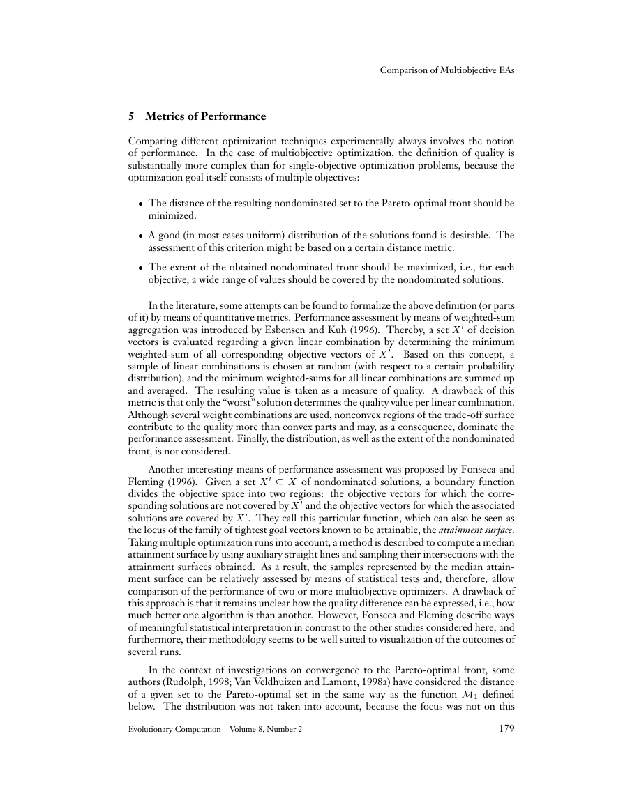
5 Metrics of Performance
Comparing different optimization techniques experimentally always involves the notion
of performance.
In the case of multiobjective optimization, the definition of quality is
substantially more complex than for single-objective optimization problems, because the
optimization goal itself consists of multiple objectives:
The distance of the resulting nondominated set to the Pareto-optimal front should be
minimized.
A good (in most cases uniform) distribution of the solutions found is desirable. The
assessment of this criterion might be based on a certain distance metric.
The extent of the obtained nondominated front should be maximized, i.e., for each
objective, a wide range of values should be covered by the nondominated solutions.
In the literature, some attempts can be found to formalize the above definition (or parts
of it) by means of quantitative metrics. Performance assessment by means of weighted-sum
aggregation was introduced by Esbensen and Kuh (1996). Thereby, a set X � of decision
vectors is evaluated regarding a given linear combination by determining the minimum
weighted-sum of all corresponding objective vectors of X �. Based on this concept, a
sample of linear combinations is chosen at random (with respect to a certain probability
distribution), and the minimum weighted-sums for all linear combinations are summed up
and averaged. The resulting value is taken as a measure of quality. A drawback of this
metric is that only the “worst” solution determines the quality value per linear combination.
Although several weight combinations are used, nonconvex regions of the trade-off surface
contribute to the quality more than convex parts and may, as a consequence, dominate the
performance assessment. Finally, the distribution, as well as the extent of the nondominated
front, is not considered.
Another interesting means of performance assessment was proposed by Fonseca and
Fleming (1996). Given a set X � X of nondominated solutions, a boundary function
divides the objective space into two regions: the objective vectors for which the corre-
sponding solutions are not covered by X � and the objective vectors for which the associated
solutions are covered by X �. They call this particular function, which can also be seen as
the locus of the family of tightest goal vectors known to be attainable, the attainment surface.
Taking multiple optimization runs into account, a method is described to compute a median
attainment surface by using auxiliary straight lines and sampling their intersections with the
attainment surfaces obtained. As a result, the samples represented by the median attain-
ment surface can be relatively assessed by means of statistical tests and, therefore, allow
comparison of the performance of two or more multiobjective optimizers. A drawback of
this approach is that it remains unclear how the quality difference can be expressed, i.e., how
much better one algorithm is than another. However, Fonseca and Fleming describe ways
of meaningful statistical interpretation in contrast to the other studies considered here, and
furthermore, their methodology seems to be well suited to visualization of the outcomes of
several runs.
In the context of investigations on convergence to the Pareto-optimal front, some
authors (Rudolph, 1998; Van Veldhuizen and Lamont, 1998a) have considered the distance
of a given set to the Pareto-optimal set in the same way as the function M� defined
below. The distribution was not taken into account, because the focus was not on this
Evolutionary Computation Volume 8, Number 2
179
�
E. Zitzler, K. Deb, and L. Thiele
matter. However, in comparative studies, distance alone is not sufficient for performance
evaluation, since extremely differently distributed fronts may have the same distance to the
Pareto-optimal front.
Two complementary metrics of performance were presented in Zitzler and Thiele
(1998, 1999). On one hand, the size of the dominated area in the objective space is
taken under consideration; on the other hand, a pair of nondominated sets is compared by
calculating the fraction of each set that is covered by the other set. The area combines all
three criteria (distance, distribution, and extent) into one, and therefore, sets differing in
more than one criterion may not be distinguished. The second metric is in some way similar
to the comparison methodology proposed in Fonseca and Fleming (1996). It can be used
to show that the outcomes of an algorithm dominate the outcomes of another algorithm,
although, it does not tell how much better it is.� We give its definition here, because it is
used in the remainder of this paper.
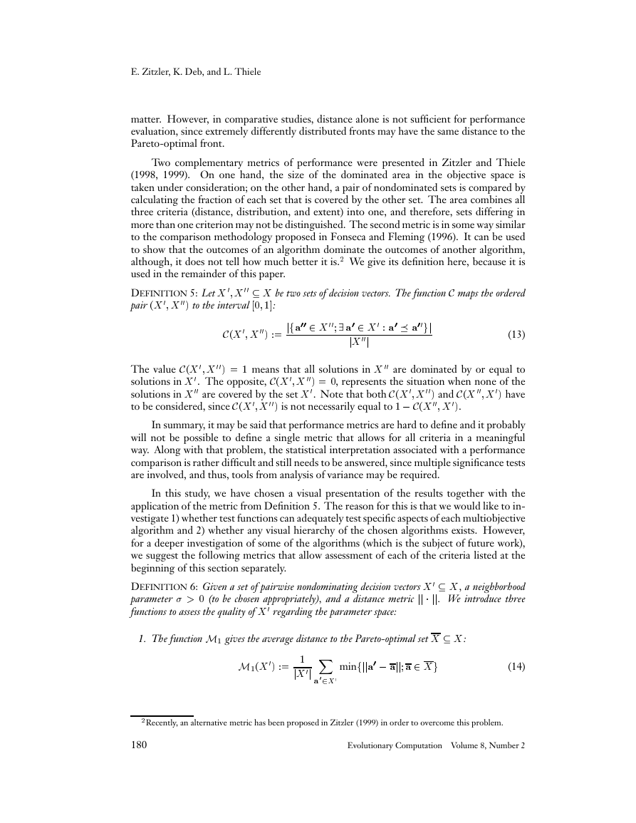
DEFINITION 5: Let X � X �� X be two sets of decision vectors. The function C maps the ordered
pair X � X �� to the interval � �:
CX � X ��
jfa�� � X �� a� � X � a� a� �gj
jX ��j
(13)
The value CX � X �� � means that all solutions in X �� are dominated by or equal to
solutions in X �. The opposite, CX � X �� �, represents the situation when none of the
solutions in X �� are covered by the set X �. Note that both CX � X �� and CX �� X � have
to be considered, since CX � X �� is not necessarily equal to � CX �� X �.
In summary, it may be said that performance metrics are hard to define and it probably
will not be possible to define a single metric that allows for all criteria in a meaningful
way. Along with that problem, the statistical interpretation associated with a performance
comparison is rather difficult and still needs to be answered, since multiple significance tests
are involved, and thus, tools from analysis of variance may be required.
In this study, we have chosen a visual presentation of the results together with the
application of the metric from Definition 5. The reason for this is that we would like to in-
vestigate 1) whether test functions can adequately test specific aspects of each multiobjective
algorithm and 2) whether any visual hierarchy of the chosen algorithms exists. However,
for a deeper investigation of some of the algorithms (which is the subject of future work),
we suggest the following metrics that allow assessment of each of the criteria listed at the
beginning of this section separately.
DEFINITION 6: Given a set of pairwise nondominating decision vectors X � X, a neighborhood
parameter � (to be chosen appropriately), and a distance metric jj jj. We introduce three
functions to assess the quality of X � regarding the parameter space:
1. The function M� gives the average distance to the Pareto-optimal set X X:
M�X �
�
jX �j Xa
�
�X �
minfjja� ajj a � Xg
(14)
�Recently, an alternative metric has been proposed in Zitzler (1999) in order to overcome this problem.
180
Evolutionary Computation Volume 8, Number 2
�


 2023年江西萍乡中考道德与法治真题及答案.doc
 2012年重庆南川中考生物真题及答案.doc
 2013年江西师范大学地理学综合及文艺理论基础考研真题.doc
 2020年四川甘孜小升初语文真题及答案I卷.doc
 2020年注册岩土工程师专业基础考试真题及答案.doc
 2023-2024学年福建省厦门市九年级上学期数学月考试题及答案.doc
 2021-2022学年辽宁省沈阳市大东区九年级上学期语文期末试题及答案.doc
 2022-2023学年北京东城区初三第一学期物理期末试卷及答案.doc
 2018上半年江西教师资格初中地理学科知识与教学能力真题及答案.doc
 2012年河北国家公务员申论考试真题及答案-省级.doc
 2020-2021学年江苏省扬州市江都区邵樊片九年级上学期数学第一次质量检测试题及答案.doc
 2022下半年黑龙江教师资格证中学综合素质真题及答案.doc