Foundations and Trends R in
Machine Learning
Vol. 1, Nos. 1–2 (2008) 1–305
c 2008 M. J. Wainwright and M. I. Jordan
DOI: 10.1561/2200000001
Graphical Models, Exponential Families, and
Variational Inference
Martin J. Wainwright1 and Michael I. Jordan2
1 Department of Statistics, and Department of Electrical Engineering and
Computer Science, University of California, Berkeley 94720, USA,
wainwrig@stat.berkeley.edu
2 Department of Statistics, and Department of Electrical Engineering and
Computer Science, University of California, Berkeley 94720, USA,
jordan@stat.berkeley.edu
Abstract
The formalism of probabilistic graphical models provides a unifying
framework for capturing complex dependencies among random
variables, and building large-scale multivariate statistical models.
Graphical models have become a focus of research in many statisti-
cal, computational and mathematical fields, including bioinformatics,
communication theory, statistical physics, combinatorial optimiza-
tion, signal and image processing, information retrieval and statistical
machine learning. Many problems that arise in specific instances —
including the key problems of computing marginals and modes of
probability distributions — are best studied in the general setting.
Working with exponential family representations, and exploiting the
conjugate duality between the cumulant function and the entropy
for exponential families, we develop general variational representa-
tions of the problems of computing likelihoods, marginal probabili-
ties and most probable configurations. We describe how a wide variety
�
of algorithms — among them sum-product, cluster variational meth-
ods, expectation-propagation, mean field methods, max-product and
linear programming relaxation, as well as conic programming relax-
ations — can all be understood in terms of exact or approximate forms
of these variational representations. The variational approach provides
a complementary alternative to Markov chain Monte Carlo as a general
source of approximation methods for inference in large-scale statistical
models.
�
1
Introduction
Graphical models bring together graph theory and probability theory
in a powerful formalism for multivariate statistical modeling. In vari-
ous applied fields including bioinformatics, speech processing, image
processing and control theory, statistical models have long been for-
mulated in terms of graphs, and algorithms for computing basic statis-
tical quantities such as likelihoods and score functions have often been
expressed in terms of recursions operating on these graphs; examples
include phylogenies, pedigrees, hidden Markov models, Markov random
fields, and Kalman filters. These ideas can be understood, unified, and
generalized within the formalism of graphical models. Indeed, graphi-
cal models provide a natural tool for formulating variations on these
classical architectures, as well as for exploring entirely new families of
statistical models. Accordingly, in fields that involve the study of large
numbers of interacting variables, graphical models are increasingly in
evidence.
Graph theory plays an important role in many computationally ori-
ented fields, including combinatorial optimization, statistical physics,
and economics. Beyond its use as a language for formulating models,
graph theory also plays a fundamental role in assessing computational
3
�
4 Introduction
complexity and feasibility. In particular, the running time of an algo-
rithm or the magnitude of an error bound can often be characterized
in terms of structural properties of a graph. This statement is also true
in the context of graphical models. Indeed, as we discuss, the com-
putational complexity of a fundamental method known as the junction
tree algorithm — which generalizes many of the recursive algorithms on
graphs cited above — can be characterized in terms of a natural graph-
theoretic measure of interaction among variables. For suitably sparse
graphs, the junction tree algorithm provides a systematic solution to
the problem of computing likelihoods and other statistical quantities
associated with a graphical model.
Unfortunately, many graphical models of practical interest are not
“suitably sparse,” so that the junction tree algorithm no longer provides
a viable computational framework. One popular source of methods for
attempting to cope with such cases is the Markov chain Monte Carlo
(MCMC) framework, and indeed there is a significant literature on the
application of MCMC methods to graphical models [e.g., 28, 93, 202].
Our focus in this survey is rather different: we present an alternative
computational methodology for statistical inference that is based on
variational methods. These techniques provide a general class of alter-
natives to MCMC, and have applications outside of the graphical model
framework. As we will see, however, they are particularly natural in
their application to graphical models, due to their relationships with
the structural properties of graphs.
The phrase “variational” itself is an umbrella term that refers to var-
ious mathematical tools for optimization-based formulations of prob-
lems, as well as associated techniques for their solution. The general
idea is to express a quantity of interest as the solution of an opti-
mization problem. The optimization problem can then be “relaxed”
in various ways, either by approximating the function to be optimized
or by approximating the set over which the optimization takes place.
Such relaxations, in turn, provide a means of approximating the original
quantity of interest.
The roots of both MCMC methods and variational methods lie
in statistical physics. Indeed, the successful deployment of MCMC
methods in statistical physics motivated and predated their entry into
�
5
statistics. However, the development of MCMC methodology specif-
ically designed for statistical problems has played an important role
in sparking widespread application of such methods in statistics [88].
A similar development in the case of variational methodology would be
of significant interest. In our view, the most promising avenue toward
a variational methodology tuned to statistics is to build on existing
links between variational analysis and the exponential family of distri-
butions [4, 11, 43, 74]. Indeed, the notions of convexity that lie at the
heart of the statistical theory of the exponential family have immediate
implications for the design of variational relaxations. Moreover, these
variational relaxations have particularly interesting algorithmic conse-
quences in the setting of graphical models, where they again lead to
recursions on graphs.
Thus, we present a story with three interrelated themes. We begin
in Section 2 with a discussion of graphical models, providing both an
overview of the general mathematical framework, and also presenting
several specific examples. All of these examples, as well as the majority
of current applications of graphical models, involve distributions in the
exponential family. Accordingly, Section 3 is devoted to a discussion
of exponential families, focusing on the mathematical links to convex
analysis, and thus anticipating our development of variational meth-
ods. In particular, the principal object of interest in our exposition
is a certain conjugate dual relation associated with exponential fam-
ilies. From this foundation of conjugate duality, we develop a gen-
eral variational representation for computing likelihoods and marginal
probabilities in exponential families. Subsequent sections are devoted
to the exploration of various instantiations of this variational princi-
ple, both in exact and approximate forms, which in turn yield various
algorithms for computing exact and approximate marginal probabili-
ties, respectively. In Section 4, we discuss the connection between the
Bethe approximation and the sum-product algorithm, including both
its exact form for trees and approximate form for graphs with cycles.
We also develop the connections between Bethe-like approximations
and other algorithms, including generalized sum-product, expectation-
propagation and related moment-matching methods. In Section 5, we
discuss the class of mean field methods, which arise from a qualitatively
�
6 Introduction
different approximation to the exact variational principle, with the
added benefit of generating lower bounds on the likelihood. In Section 6,
we discuss the role of variational methods in parameter estimation,
including both the fully observed and partially observed cases, as well
as both frequentist and Bayesian settings. Both Bethe-type and mean
field methods are based on nonconvex optimization problems, which
typically have multiple solutions. In contrast, Section 7 discusses vari-
ational methods based on convex relaxations of the exact variational
principle, many of which are also guaranteed to yield upper bounds on
the log likelihood. Section 8 is devoted to the problem of mode compu-
tation, with particular emphasis on the case of discrete random vari-
ables, in which context computing the mode requires solving an integer
programming problem. We develop connections between (reweighted)
max-product algorithms and hierarchies of linear programming relax-
ations. In Section 9, we discuss the broader class of conic programming
relaxations, and show how they can be understood in terms of semidef-
inite constraints imposed via moment matrices. We conclude with a
discussion in Section 10.
The scope of this survey is limited in the following sense: given a dis-
tribution represented as a graphical model, we are concerned with the
problem of computing marginal probabilities (including likelihoods), as
well as the problem of computing modes. We refer to such computa-
tional tasks as problems of “probabilistic inference,” or “inference” for
short. As with presentations of MCMC methods, such a limited focus
may appear to aim most directly at applications in Bayesian statis-
tics. While Bayesian statistics is indeed a natural terrain for deploying
many of the methods that we present here, we see these methods as
having applications throughout statistics, within both the frequentist
and Bayesian paradigms, and we indicate some of these applications at
various junctures in the survey.
�
2
Background
We begin with background on graphical models. The key idea is that of
factorization: a graphical model consists of a collection of probability
distributions that factorize according to the structure of an underly-
ing graph. Here, we are using the terminology “distribution” loosely;
our notation p should be understood as a mass function (density with
respect to counting measure) in the discrete case, and a density with
respect to Lebesgue measure in the continuous case. Our focus in this
section is the interplay between probabilistic notions such as conditional
independence on one hand, and on the other hand, graph-theoretic
notions such as cliques and separation.
2.1 Probability Distributions on Graphs
We begin by describing the various types of graphical formalisms that
are useful. A graph G = (V, E) is formed by a collection of vertices
V = {1,2, . . . , m}, and a collection of edges E ⊂ V × V . Each edge con-
sists of a pair of vertices s, t ∈ E, and may either be undirected, in
which case there is no distinction between edge (s, t) and edge (t, s), or
directed, in which case we write (s → t) to indicate the direction. See
Appendix A.1 for more background on graphs and their properties.
7
�
8 Background
In order to define a graphical model, we associate with each vertex
s ∈ V a random variable Xs taking values in some space Xs. Depend-
ing on the application, this state space Xs may either be continuous,
(e.g., Xs = R) or discrete (e.g., Xs = {0,1, . . . , r − 1}). We use lower-
case letters (e.g., xs ∈ Xs) to denote particular elements of Xs, so that
the notation {Xs = xs} corresponds to the event that the random
variable Xs takes the value xs ∈ Xs. For any subset A of the vertex
set V , we define the subvector XA := (Xs, s ∈ A), with the notation
xA := (xs, s ∈ A) corresponding to the analogous quantity for values
of the random vector XA. Similarly, we define ⊗s∈AXs to be the Carte-
sian product of the state spaces for each of the elements of XA.
2.1.1 Directed Graphical Models
Given a directed graph with edges (s → t), we say that t is a child of
s, or conversely, that s is a parent of t. For any vertex s ∈ V , let π(s)
denote the set of all parents of given node s ∈ V . (If a vertex s has
no parents, then the set π(s) should be understood to be empty.) A
directed cycle is a sequence (s1, s2, . . . , sk) such that (si → si+1) ∈ E for
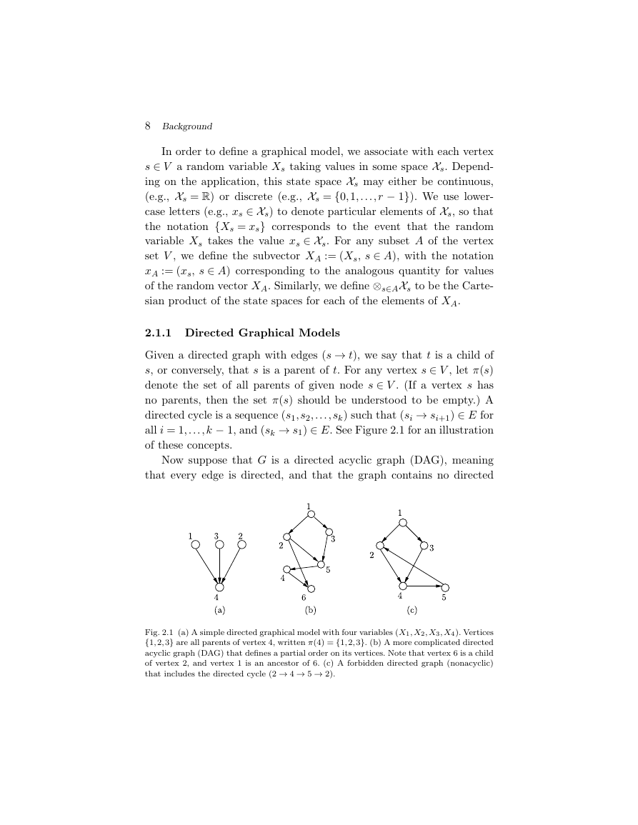
all i = 1, . . . , k − 1, and (sk → s1) ∈ E. See Figure 2.1 for an illustration
of these concepts.
Now suppose that G is a directed acyclic graph (DAG), meaning
that every edge is directed, and that the graph contains no directed
Fig. 2.1 (a) A simple directed graphical model with four variables (X1, X2, X3, X4). Vertices
{1,2,3} are all parents of vertex 4, written π(4) = {1,2,3}. (b) A more complicated directed
acyclic graph (DAG) that defines a partial order on its vertices. Note that vertex 6 is a child
of vertex 2, and vertex 1 is an ancestor of 6. (c) A forbidden directed graph (nonacyclic)
that includes the directed cycle (2 → 4 → 5 → 2).
�




 2023年江西萍乡中考道德与法治真题及答案.doc
 2012年重庆南川中考生物真题及答案.doc
 2013年江西师范大学地理学综合及文艺理论基础考研真题.doc
 2020年四川甘孜小升初语文真题及答案I卷.doc
 2020年注册岩土工程师专业基础考试真题及答案.doc
 2023-2024学年福建省厦门市九年级上学期数学月考试题及答案.doc
 2021-2022学年辽宁省沈阳市大东区九年级上学期语文期末试题及答案.doc
 2022-2023学年北京东城区初三第一学期物理期末试卷及答案.doc
 2018上半年江西教师资格初中地理学科知识与教学能力真题及答案.doc
 2012年河北国家公务员申论考试真题及答案-省级.doc
 2020-2021学年江苏省扬州市江都区邵樊片九年级上学期数学第一次质量检测试题及答案.doc
 2022下半年黑龙江教师资格证中学综合素质真题及答案.doc