计算机体系结构权威经典最新第四版教材（英文）清晰版习题答案 Computer.Architecture.-.A.Quantita....pdf-资料库

kealyn-3060509-16359647316583400500.pdf-第1页.png

第1页 / 共65页

kealyn-3060509-16359647316583400500.pdf-第2页.png

第2页 / 共65页

kealyn-3060509-16359647316583400500.pdf-第3页.png

第3页 / 共65页

kealyn-3060509-16359647316583400500.pdf-第4页.png

第4页 / 共65页

kealyn-3060509-16359647316583400500.pdf-第5页.png

第5页 / 共65页

kealyn-3060509-16359647316583400500.pdf-第6页.png

第6页 / 共65页

kealyn-3060509-16359647316583400500.pdf-第7页.png

第7页 / 共65页

kealyn-3060509-16359647316583400500.pdf-第8页.png

第8页 / 共65页

L.1 L.2 L.3 L.4 L.5 L.6 Chapter 1 Solutions Chapter 2 Solutions Chapter 3 Solutions Chapter 4 Solutions Chapter 5 Solutions Chapter 6 Solutions L-2 L-7 L-20 L-30 L-46 L-52

L Solutions to Case Study Exercises

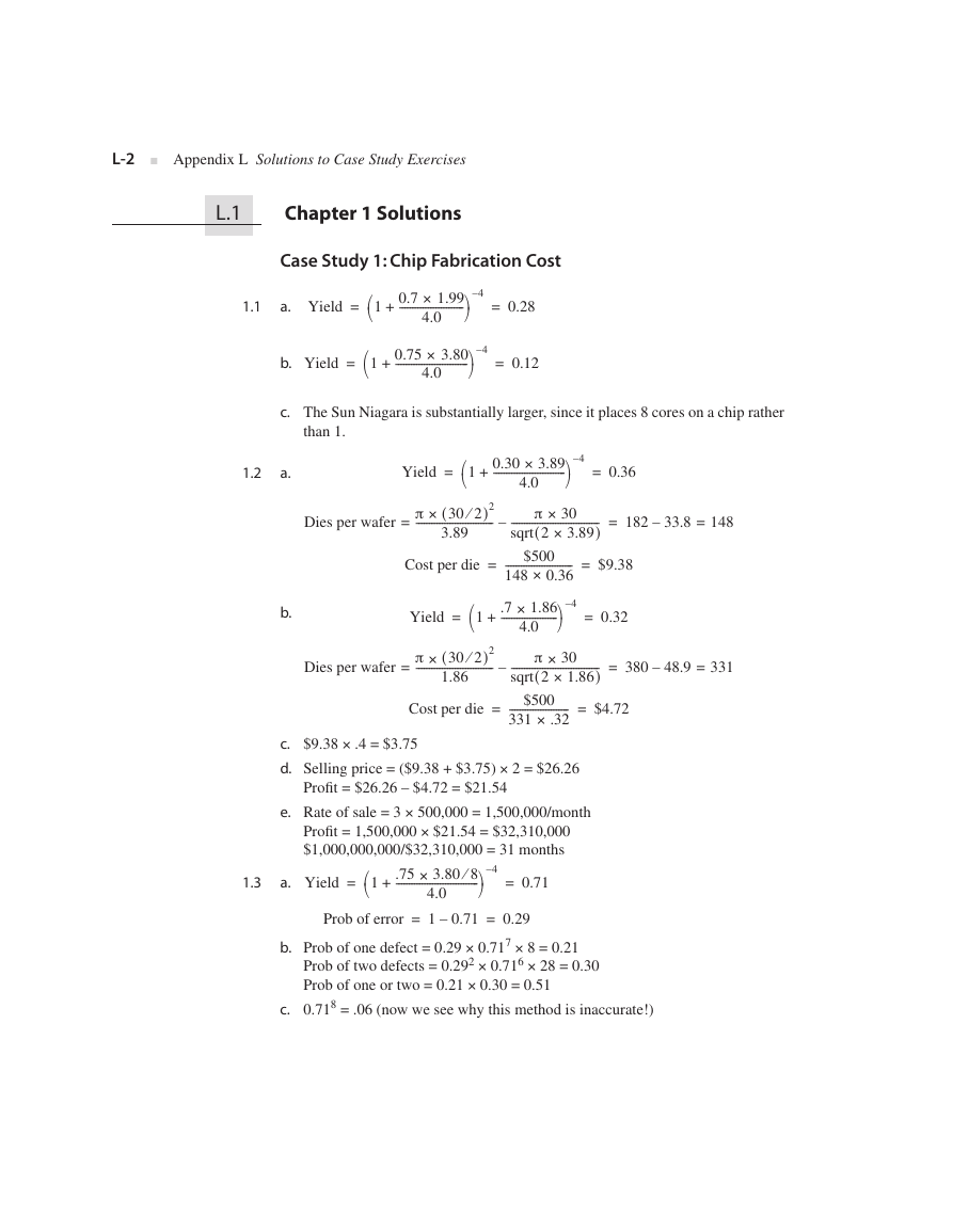
L-2 I Appendix L Solutions to Case Study Exercises L.1 Chapter 1 Solutions Case Study 1: Chip Fabrication Cost 1.1 a. Yield =  + 1 0.7 × 1.99  4– -------------------------  4.0 = 0.28 b. Yield =  + 1 0.75 × 3.80  4– ----------------------------  4.0 = 0.12 c. The Sun Niagara is substantially larger, since it places 8 cores on a chip rather than 1. 1.2 a. Yield =  + 1 0.30 × 3.89  4– ----------------------------  4.0 = 0.36 Dies per wafer = )2 π × 30 2⁄ ------------------------------ ( 3.89 – π × 30 ( ---------------------------------- ) sqrt 2 × 3.89 = 182 33.8 – = 148 Cost per die = $500 -------------------------- 148 × 0.36 = $9.38 Yield =  + 1 .7 × 1.86  4– ----------------------  4.0 = 0.32 Dies per wafer = )2 π × 30 2⁄ ------------------------------ ( 1.86 – π × 30 ( ---------------------------------- ) sqrt 2 × 1.86 = 380 48.9 – = 331 Cost per die = $500 ----------------------- 331 × .32 = $4.72 × .4 = $3.75 $9.38 × Selling price = ($9.38 + $3.75) 2 = $26.26 Proﬁt = $26.26 – $4.72 = $21.54 × 500,000 = 1,500,000/month Rate of sale = 3 × Proﬁt = 1,500,000 $21.54 = $32,310,000 $1,000,000,000/$32,310,000 = 31 months Yield = = 0.71  + 1 .75 × 3.80 8⁄  4– --------------------------------  = = Prob of error 4.0 – 1 0.71 0.29 × × 7 8 = 0.21 0.71 Prob of one defect = 0.29 × × 2 6 Prob of two defects = 0.29 0.71 28 = 0.30 × Prob of one or two = 0.21 0.30 = 0.51 8 0.71 = .06 (now we see why this method is inaccurate!) b. c. d. e. 1.3 a. b. c.

L.1 Chapter 1 Solutions I L 3 - d. e. 0.51 ⁄ 0.06 = 8.5 × × $1.50 = $200,000,000 $150 + 8.5 x x = 885,938 8-core chips, 8,416,390 chips total x × $100 – (9.5 x × $80) – 9.5 x Case Study 2: Power Consumption in Computer Systems 1.4 a. b. c. 1.5 a. × 3.7 + 2 × 7.9 = 146 x = 79 + 2 x .70 × 4.0 W .4 + 7.9 W The 7200 rpm drive takes 60 s to read/seek and 40 s idle for a particular job. × The 5400 rpm disk requires 4/3 60 s, or 80 s to do the same thing. There- fore, it is idle 20% of the time. × .6 = 6.34 W ------------------------------------------------------------ ) ( 79 W 2.3 W 7.0 W 14 KW + + = 158 b. 14 KW ---------------------------------------------------------------------- ) ( + × 7.0 W 79 W 2.3 W 2 + = 146 c. MTTF = 1 ------------------ 9 × 106 + 8 × 1 ------------ 4500 + 1 ------------------ 3 × 104 = 8 × 2000 300 ------------------------------------- + 9 × 106 = 16301 ------------------ 9 × 106 1 --------------------------- Failure rate = 9 × 106 ------------------ 16301 = 522 hours 1.6 a. See Figure L.1. SPECjbb SPECweb Sun Fire T2000 IBM x346 213 42.4 91.2 9.93 Figure L.1 Power/performance ratios. b. c. a. b. 1.7 Sun Fire T2000 More expensive servers can be more compact, allowing more computers to be stored in the same amount of space. Because real estate is so expensive, this is a huge concern. Also, power may not be the same for both systems. It can cost more to purchase a chip that is optimized for lower power consumption. 50% Power new -------------------------- Power old = )2 × F × 0.50 ) ( V × 0.50 ( -------------------------------------------------------------- V 2 × F = 0.53 = 0.125 c. = .70 ) -------------------------------- ; x x–( 1 x 2⁄+ = 60%

L-4 I Appendix L Solutions to Case Study Exercises d. Power new -------------------------- Power old = )2 × F × 0.50 ) ( V × 0.70 -------------------------------------------------------------- V 2 ( × F = 0.72 × 0.5 = 0.245 Case Study 3: The Cost of Reliability (and Failure) in Web Servers 1.8 a. b. × 14 days $1.4 million⁄day = $19.6 million $4 billion – $19.6 million = $3.98 billion Increase in total revenue: 4.8/3.9 = 1.23 In the fourth quarter, the rough estimate would be a loss of 1.23 lion = $24.1 million. × $19.6 mil- c. Losing $1.4 million × .50 = $700,000 per day. This pays for $700,000/$7,500 d. = 93 computers per day. It depends on how the 2.6 million visitors are counted. If the 2.6 million visitors are not unique, but are actually visitors each day summed across a month: 2.6 million × 8.4 = 21.84 million transactions per month. $5.38 × 21.84 million = $117 million per month. If the 2.6 million visitors are assumed to visit every day: 2.6 million × 8.4 × 31 = 677 million transactions per month. $5.38 × 677 million = $3.6 billion per month, which is clearly not the case, or else their online service would not make money. 1.9 a. FIT = 109⁄ MTTF MTTF = 109⁄ FIT = 109⁄ 100 = 10,000,000 b. Availability = MTTF --------------------------------------- MTTF MTTR + = 107 -------------------- 107 24+ = about 100% 1.10 Using the simplifying assumption that all failures are independent, we sum the probability of failure rate of all of the computers: Failure rate = 1000 × 10–7 = 10–4 = 105 -------- 109 FIT = 105, therefore MTTF = 109 -------- 105 = 104 1.11 a. Assuming that we do not repair the computers, we wait for how long it takes for 3,334 computers to fail. 3,334 × 10,000,000 = 33,340,000,000 hours b. Total cost of the decision: $1,000 × 10,000 computers = $10 million Expected beneﬁt of the decision: Gain a day of downtime for every 33,340,000,000 hours of uptime. This would save us $1.4 million each 3,858,000 years. This would deﬁnitely not be worth it.

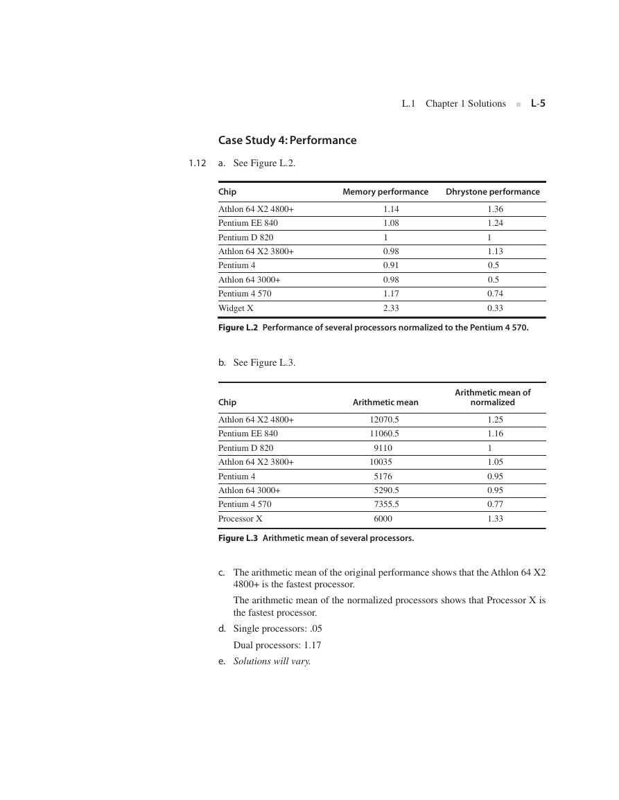
L.1 Chapter 1 Solutions I L-5 Case Study 4: Performance 1.12 a. See Figure L.2. Chip Memory performance Dhrystone performance Athlon 64 X2 4800+ Pentium EE 840 Pentium D 820 Athlon 64 X2 3800+ Pentium 4 Athlon 64 3000+ Pentium 4 570 Widget X 1.14 1.08 1 0.98 0.91 0.98 1.17 2.33 1.36 1.24 1 1.13 0.5 0.5 0.74 0.33 Figure L.2 Performance of several processors normalized to the Pentium 4 570. b. See Figure L.3. Chip Athlon 64 X2 4800+ Pentium EE 840 Pentium D 820 Athlon 64 X2 3800+ Pentium 4 Athlon 64 3000+ Pentium 4 570 Processor X Arithmetic mean Arithmetic mean of normalized 12070.5 11060.5 9110 10035 5176 5290.5 7355.5 6000 1.25 1.16 1 1.05 0.95 0.95 0.77 1.33 Figure L.3 Arithmetic mean of several processors. c. The arithmetic mean of the original performance shows that the Athlon 64 X2 4800+ is the fastest processor. The arithmetic mean of the normalized processors shows that Processor X is the fastest processor. d. Single processors: .05 Dual processors: 1.17 e. Solutions will vary.

L-6 I Appendix L Solutions to Case Study Exercises f. Dual processors gain in CPU performance (exhibited by the Dhrystone per- formance), but they do not necessarily increase in memory performance. This makes sense because, although they are doubling the processing power, dual processors do not change the memory hierarchy very much. Benchmarks that exercise the memory often do not ﬁt in the size of the cache, so doubling the cache does not help the memory benchmarks substantially. In some applica- tions, however, they could gain substantially due to the increased cache avail- able. 1.13 a. Pentium 4 570: .4 × 3,501 + .6 × 11,210 = 8,126 Athlon 64 X2 4,800+: .4 × 3,423 + .6 × 20,718 = 13,800 b. 20,718/7,621 = 2.7 c. 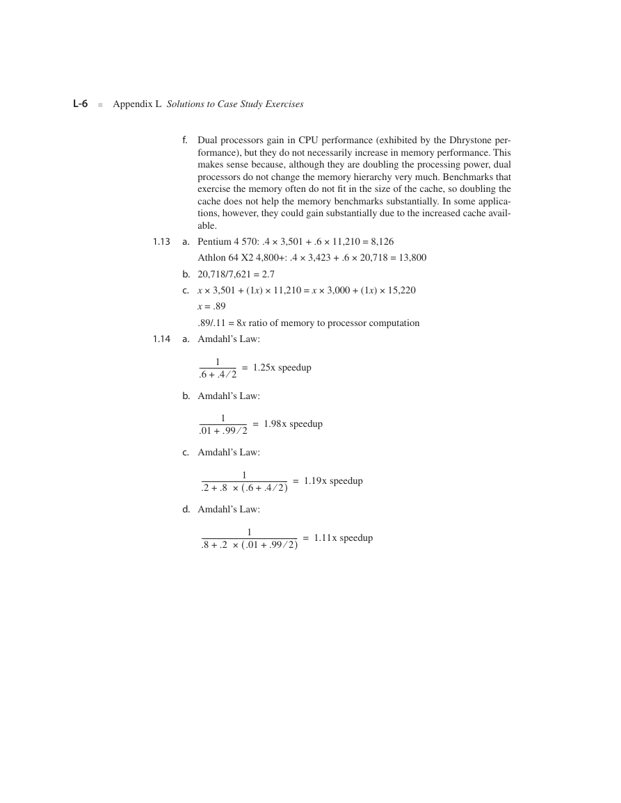x × 3,501 + (1x) × 11,210 = x × 3,000 + (1x) × 15,220 x = .89 .89/.11 = 8x ratio of memory to processor computation 1.14 a. Amdahl’s Law: 1 ---------------------- .4 2⁄ .6 + = 1.25x speedup b. Amdahl’s Law: 1 ---------------------------- .99 2⁄ .01 + = 1.98x speedup c. Amdahl’s Law: --------------------------------------------------- ) .4 2⁄ .2 1 +( .8 × .6 + = 1.19x speedup d. Amdahl’s Law: --------------------------------------------------------- ) .99 2⁄ .8 1 .2 × .01 + ( + = 1.11x speedup

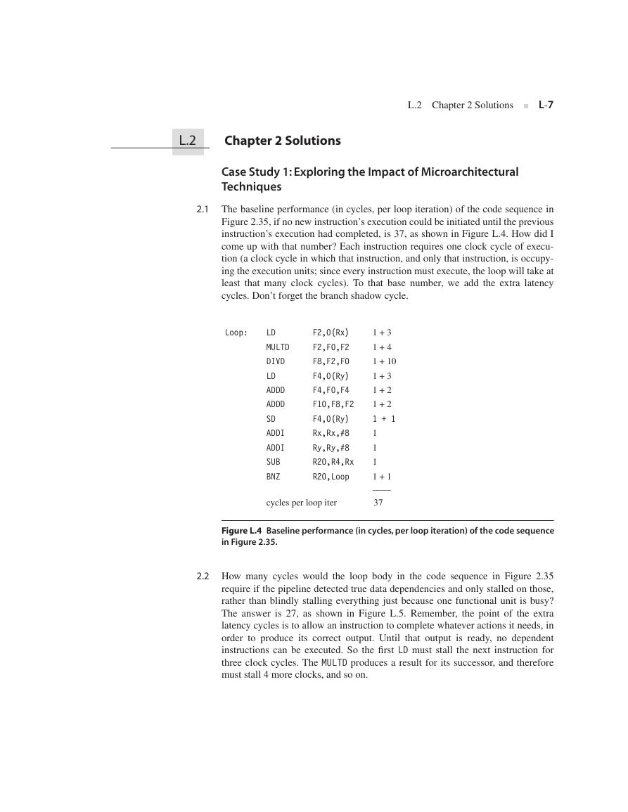
L.2 Chapter 2 Solutions I L-7 L.2 Chapter 2 Solutions Case Study 1: Exploring the Impact of Microarchitectural Techniques 2.1 The baseline performance (in cycles, per loop iteration) of the code sequence in Figure 2.35, if no new instruction’s execution could be initiated until the previous instruction’s execution had completed, is 37, as shown in Figure L.4. How did I come up with that number? Each instruction requires one clock cycle of execu- tion (a clock cycle in which that instruction, and only that instruction, is occupy- ing the execution units; since every instruction must execute, the loop will take at least that many clock cycles). To that base number, we add the extra latency cycles. Don’t forget the branch shadow cycle. Loop: LD F2,0(Rx) 1 + 3 MULTD F2,F0,F2 1 + 4 DIVD F8,F2,F0 1 + 10 LD F4,0(Ry) 1 + 3 ADDD F4,F0,F4 1 + 2 ADDD F10,F8,F2 1 + 2 SD F4,0(Ry) 1 + 1 ADDI Rx,Rx,#8 1 ADDI Ry,Ry,#8 1 SUB R20,R4,Rx 1 BNZ R20,Loop 1 + 1 ____ cycles per loop iter 37 Figure L.4 Baseline performance (in cycles, per loop iteration) of the code sequence in Figure 2.35. 2.2 How many cycles would the loop body in the code sequence in Figure 2.35 require if the pipeline detected true data dependencies and only stalled on those, rather than blindly stalling everything just because one functional unit is busy? The answer is 27, as shown in Figure L.5. Remember, the point of the extra latency cycles is to allow an instruction to complete whatever actions it needs, in order to produce its correct output. Until that output is ready, no dependent instructions can be executed. So the ﬁrst LD must stall the next instruction for three clock cycles. The MULTD produces a result for its successor, and therefore must stall 4 more clocks, and so on.

资料库

计算机体系结构权威经典最新第四版教材（英文）清晰版习题答案 Computer.Architecture.-.A.Quantita....pdf

相关推荐

课程资源

热门标签

最新资料