1.1
SOLUTIONS
Notes: The key exercises are 7 (or 11 or 12), 19–22, and 25. For brevity, the symbols R1, R2,…, stand for
row 1 (or equation 1), row 2 (or equation 2), and so on. Additional notes are at the end of the section.
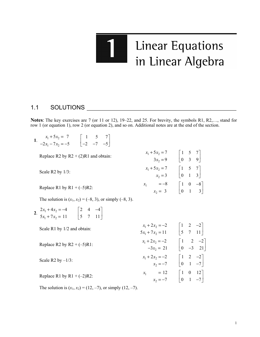
1.
x
1
x
1
+
−
5
7
x
2
x
2
=
7
= −
5
−
2
1
−
2
5
−
7
7
−
5
Replace R2 by R2 + (2)R1 and obtain:
Scale R2 by 1/3:
Replace R1 by R1 + (–5)R2:
The solution is (x1, x2) = (–8, 3), or simply (–8, 3).
2.
2
5
x
1
x
1
+
+
4
7
x
2
x
2
= −
4
=
11
2
5
4
7
−
4
11
+
x
1
+
x
1
5
3
5
x
1
=
x
7
2
=
x
9
2
=
x
7
2
=
x
3
2
= −
8
=
3
x
2
Scale R1 by 1/2 and obtain:
Replace R2 by R2 + (–5)R1:
Scale R2 by –1/3:
Replace R1 by R1 + (–2)R2:
The solution is (x1, x2) = (12, –7), or simply (12, –7).
+
x
2
2
+
x
7
2
+
x
2
2
−
x
3
2
+
x
2
2
x
2
x
1
x
5
1
x
1
x
1
x
1
x
2
= −
2
=
11
= −
2
=
21
= −
2
= −
7
=
12
= −
7
1
0
1
0
1
0
1
5
1
0
1
0
1
0
5
3
5
1
0
1
7
9
7
3
−
8
3
2
7
2
−
3
2
1
0
1
−
2
11
−
2
21
−
2
−
7
12
−
7
1
�
2 CHAPTER 1
• Linear Equations in Linear Algebra
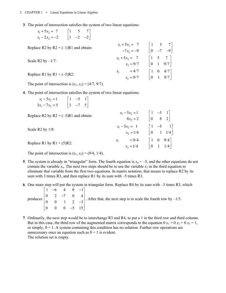
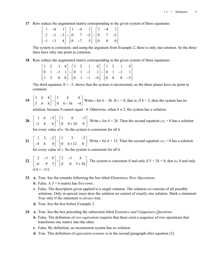
3. The point of intersection satisfies the system of two linear equations:
x
1
x
1
+
−
5
2
x
2
x
2
=
7
= −
2
1
1
5
−
2
7
−
2
Replace R2 by R2 + (–1)R1 and obtain:
Scale R2 by –1/7:
Replace R1 by R1 + (–5)R2:
The point of intersection is (x1, x2) = (4/7, 9/7).
x
1
+
x
5
2
−
x
7
2
+
x
5
2
x
2
x
1
x
1
x
2
=
7
= −
9
=
7
=
9/7
=
4/7
=
9/7
4. The point of intersection satisfies the system of two linear equations:
x
1
x
1
3
−
−
5
7
x
2
x
2
=
1
=
5
1
3
−
5
−
7
1
5
Replace R2 by R2 + (–3)R1 and obtain:
x
1
−
Scale R2 by 1/8:
Replace R1 by R1 + (5)R2:
The point of intersection is (x1, x2) = (9/4, 1/4).
5
8
x
2
x
2
x
2
x
2
=
=
=
=
=
1
=
2
1
1/4
9/4
1/4
−
5
x
1
x
1
x
2
1
0
1
0
1
0
1
0
1
0
1
0
5
−
7
5
1
0
1
7
−
9
7
9/7
4/7
9/7
−
1
5
2
8
−
1
5
1 1/4
9/4
1/4
0
1
5. The system is already in “triangular” form. The fourth equation is x4 = –5, and the other equations do not
contain the variable x4. The next two steps should be to use the variable x3 in the third equation to
eliminate that variable from the first two equations. In matrix notation, that means to replace R2 by its
sum with 3 times R3, and then replace R1 by its sum with –5 times R3.
6. One more step will put the system in triangular form. Replace R4 by its sum with –3 times R3, which
produces
1
0
0
0
−
6
2
0
0
4
−
7
1
0
0
0
2
−
5
−
1
4
−
3
15
. After that, the next step is to scale the fourth row by –1/5.
7. Ordinarily, the next step would be to interchange R3 and R4, to put a 1 in the third row and third column.
But in this case, the third row of the augmented matrix corresponds to the equation 0 x1 + 0 x2 + 0 x3 = 1,
or simply, 0 = 1. A system containing this condition has no solution. Further row operations are
unnecessary once an equation such as 0 = 1 is evident.
The solution set is empty.
�
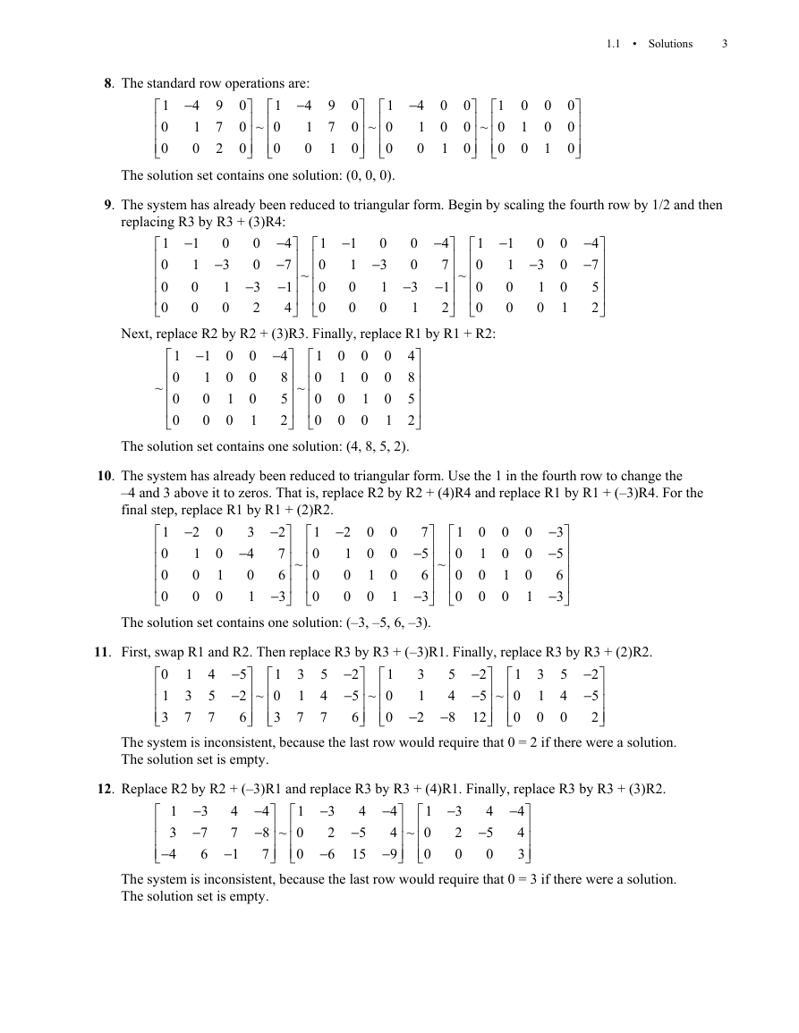
8. The standard row operations are:
−
4
1
0
0
1
0 ~ 0
0
0
The solution set contains one solution: (0, 0, 0).
0
1
0 ~ 0
0
0
−
4
1
0
9
7
1
1
0
0
9
7
2
1.1
• Solutions
3
−
4
1
0
0
0
1
0
1
0 ~ 0
0
0
0
1
0
0
0
1
0
0
0
9. The system has already been reduced to triangular form. Begin by scaling the fourth row by 1/2 and then
replacing R3 by R3 + (3)R4:
−
4
−
7
−
1
4
0
−
3
1
0
−
1
1
0
0
0
0
−
3
2
1
0
0
0
~
1
0
0
0
−
1
1
0
0
0
−
3
1
0
0
0
−
3
1
−
4
7
−
1
2
~
1
0
0
0
−
1
1
0
0
0
−
3
1
0
0
0
0
1
−
4
−
7
5
2
Next, replace R2 by R2 + (3)R3. Finally, replace R1 by R1 + R2:
~
1
0
0
0
4
8
5
2
The solution set contains one solution: (4, 8, 5, 2).
0
0
0
1
0
1
0
0
0
0
1
0
0
0
1
0
0
0
0
1
1
0
0
0
−
4
8
5
2
−
1
1
0
0
~
10. The system has already been reduced to triangular form. Use the 1 in the fourth row to change the
–4 and 3 above it to zeros. That is, replace R2 by R2 + (4)R4 and replace R1 by R1 + (–3)R4. For the
final step, replace R1 by R1 + (2)R2.
−
2
1
0
0
7
−
5
6
−
3
The solution set contains one solution: (–3, –5, 6, –3).
−
3
−
5
6
−
3
−
2
1
0
0
3
−
4
0
1
−
2
7
6
−
3
0
0
1
0
0
0
1
0
0
0
0
1
0
0
0
1
0
1
0
0
0
0
1
0
1
0
0
0
1
0
0
0
1
0
0
0
~
~
11. First, swap R1 and R2. Then replace R3 by R3 + (–3)R1. Finally, replace R3 by R3 + (2)R2.
0
1
3
1
3
7
4
5
7
−
5
1
−
2 ~ 0
6
3
3
1
7
5
4
7
−
2
1
−
5 ~ 0
6
0
3
1
−
2
5
4
−
8
−
2
1
−
5 ~ 0
12
0
3
1
0
5
4
0
−
2
−
5
2
The system is inconsistent, because the last row would require that 0 = 2 if there were a solution.
The solution set is empty.
12. Replace R2 by R2 + (–3)R1 and replace R3 by R3 + (4)R1. Finally, replace R3 by R3 + (3)R2.
1
3
−
4
−
3
−
7
6
4
7
−
1
−
1
4
−
8 ~ 0
7
0
−
3
2
−
6
4
−
5
15
−
4
1
4 ~ 0
−
9
0
−
3
2
0
4
−
5
0
−
4
4
3
The system is inconsistent, because the last row would require that 0 = 3 if there were a solution.
The solution set is empty.
�
4 CHAPTER 1
• Linear Equations in Linear Algebra
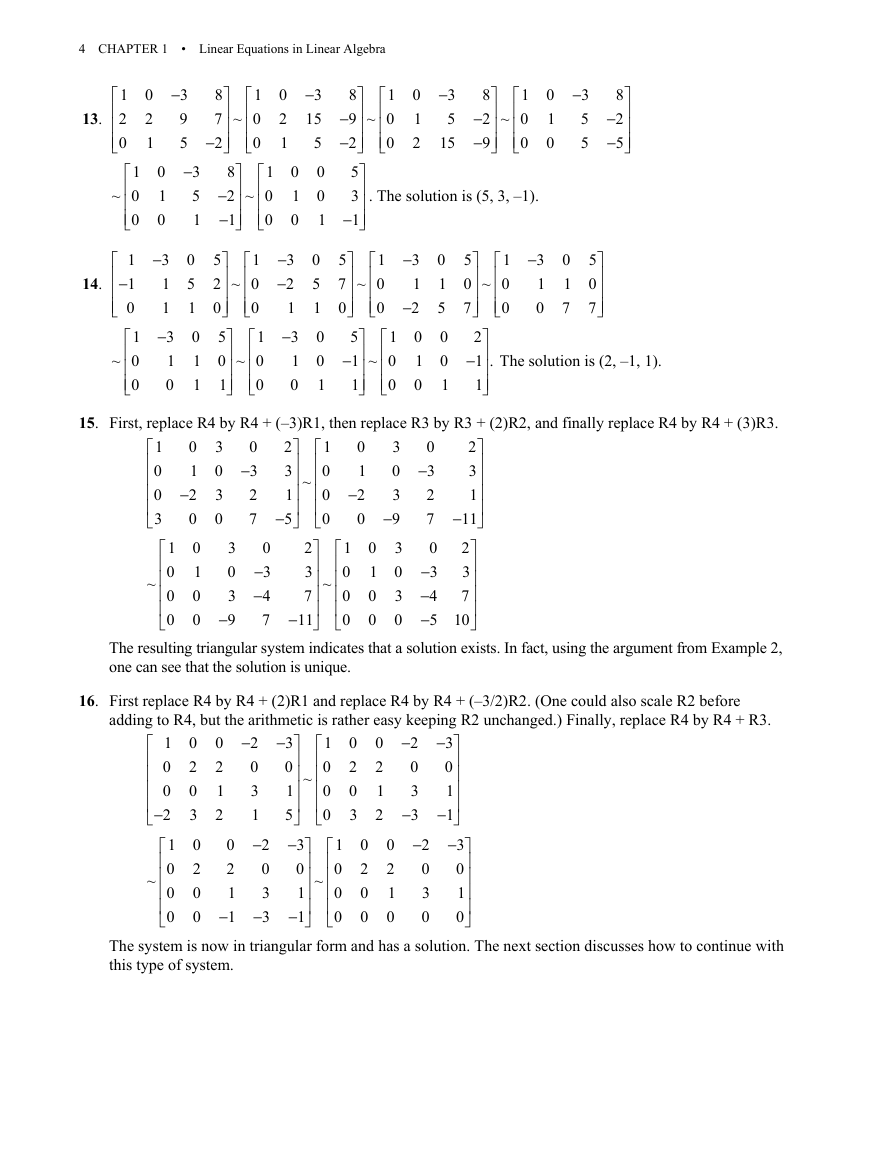
13.
14.
1
2
0
1
~ 0
0
1
−
1
0
1
~ 0
0
0
2
1
−
3
9
5
−
3
5
1
8
1
7 ~ 0
−
2
0
8
1
−
2 ~ 0
−
1
0
0
1
0
−
3
1
1
−
3
1
0
0
5
1
0
1
1
1
5
2 ~ 0
0
0
5
1
0 ~ 0
1
0
0
2
1
0
1
0
−
3
−
2
1
−
3
1
0
−
3
15
5
0
0
1
0
5
1
0
0
1
0
1
2
−
3
5
15
8
1
−
2 ~ 0
−
9
0
0
1
0
−
3
5
5
8
−
2
−
5
. The solution is (5, 3, –1).
8
1
−
9 ~ 0
−
2
0
5
3
−
1
−
3
1
0
0
1
7
5
0
7
1
5
7 ~ 0
0
0
5
1
−
1 ~ 0
1
0
−
3
1
−
2
0
1
0
0
1
5
0
0
1
1
5
0 ~ 0
7
0
2
−
1 .
1
The solution is (2, –1, 1).
15. First, replace R4 by R4 + (–3)R1, then replace R3 by R3 + (2)R2, and finally replace R4 by R4 + (3)R3.
1
0
0
3
~
1
0
0
0
0
1
−
2
0
0
1
0
0
3
0
3
0
0
−
3
2
7
3
0
3
−
9
0
−
3
−
4
7
2
3
1
−
5
~
2
3
7
−
11
1
0
0
0
~
0
1
−
2
0
1
0
0
0
0
1
0
0
3
0
3
−
9
3
0
3
0
0
−
3
2
7
0
−
3
−
4
−
5
2
3
1
−
11
2
3
7
10
The resulting triangular system indicates that a solution exists. In fact, using the argument from Example 2,
one can see that the solution is unique.
16. First replace R4 by R4 + (2)R1 and replace R4 by R4 + (–3/2)R2. (One could also scale R2 before
adding to R4, but the arithmetic is rather easy keeping R2 unchanged.) Finally, replace R4 by R4 + R3.
~
1
0
0
−
2
1
0
0
0
0
2
0
3
0
2
0
0
0
2
1
2
0
2
1
−
1
−
2
0
3
1
−
2
0
3
−
3
~
−
3
0
1
5
−
3
0
1
−
1
1
0
0
0
~
1
0
0
0
0
2
0
3
0
2
1
2
0
2
0
0
0
2
1
0
−
2
0
3
−
3
−
2
0
3
0
−
3
0
1
−
1
−
3
0
1
0
The system is now in triangular form and has a solution. The next section discusses how to continue with
this type of system.
�
1
2
−
1
−
4
−
1
−
3
1
1
−
3 ~ 0
4
0
−
4
7
−
7
1
1
−
5 ~ 0
5
0
−
4
7
0
1
−
5
0
17. Row reduce the augmented matrix corresponding to the given system of three equations:
1.1
• Solutions
5
The system is consistent, and using the argument from Example 2, there is only one solution. So the three
lines have only one point in common.
18. Row reduce the augmented matrix corresponding to the given system of three equations:
1
0
1
2
1
3
1
−
1
0
4
1
1 ~ 0
0
0
2
1
1
1
−
1
−
1
4
1
1 ~ 0
−
4
0
2
1
0
1
−
1
0
4
1
−
5
The third equation, 0 = –5, shows that the system is inconsistent, so the three planes have no point in
common.
19.
20.
21.
22.
4
8
h
6
1
3
solution, because 0 cannot equal –4. Otherwise, when h ≠ 2, the system has a solution.
Write c for 6 – 3h. If c = 0, that is, if h = 2, then the system has no
h
−
h
6 3
4
−
4
1
0
~
h
4
1
−
2
for every value of c. So the system is consistent for all h.
h
+
4 2
1
0
~
h
−
3
0
−
3
6
.
Write c for 4 + 2h. Then the second equation cx2 = 0 has a solution
−
2
8
3
h
1
−
4
for every value of c. So the system is consistent for all h.
3
+
12
1
0
~
h
.
−
2
0
Write c for h + 12. Then the second equation cx2 = 0 has a solution
−
3
9
2
−
6
if h = –5/3.
h
5
~
2
0
−
3
0
h
+
h
5 3
.
The system is consistent if and only if 5 + 3h = 0, that is, if and only
23. a. True. See the remarks following the box titled Elementary Row Operations.
b. False. A 5 × 6 matrix has five rows.
c. False. The description given applied to a single solution. The solution set consists of all possible
solutions. Only in special cases does the solution set consist of exactly one solution. Mark a statement
True only if the statement is always true.
d. True. See the box before Example 2.
24. a. True. See the box preceding the subsection titled Existence and Uniqueness Questions.
b. False. The definition of row equivalent requires that there exist a sequence of row operations that
transforms one matrix into the other.
c. False. By definition, an inconsistent system has no solution.
d. True. This definition of equivalent systems is in the second paragraph after equation (2).
�
6 CHAPTER 1
• Linear Equations in Linear Algebra
25.
1
0
−
2
−
4
3
5
7
−
5
−
9
g
h
k
1
~ 0
0
−
4
3
−
3
7
−
5
5
g
h
+
2
g
1
~ 0
0
k
−
4
3
0
7
−
5
0
g
h
g
2
+
h
+
k
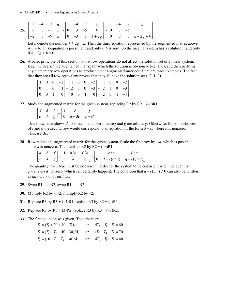
Let b denote the number k + 2g + h. Then the third equation represented by the augmented matrix above
is 0 = b. This equation is possible if and only if b is zero. So the original system has a solution if and only
if k + 2g + h = 0.
26. A basic principle of this section is that row operations do not affect the solution set of a linear system.
Begin with a simple augmented matrix for which the solution is obviously (–2, 1, 0), and then perform
any elementary row operations to produce other augmented matrices. Here are three examples. The fact
that they are all row equivalent proves that they all have the solution set (–2, 1, 0).
1
0
0
0
1
0
0
0
1
−
2
1
1 ~ 2
0
0
0
1
0
0
0
1
−
1
2
−
3 ~ 2
0
2
0
1
0
0
0
1
−
2
−
3
−
4
27. Study the augmented matrix for the given system, replacing R2 by R2 + (–c)R1:
1
c
3
d
f
g
~
1
0
3
−
c
3
d
f
−
g cf
This shows that shows d – 3c must be nonzero, since f and g are arbitrary. Otherwise, for some choices
of f and g the second row would correspond to an equation of the form 0 = b, where b is nonzero.
Thus d ≠ 3c.
28. Row reduce the augmented matrix for the given system. Scale the first row by 1/a, which is possible
The quantity d – c(b/a) must be nonzero, in order for the system to be consistent when the quantity
g – c( f /a) is nonzero (which can certainly happen). The condition that d – c(b/a) ≠ 0 can also be written
as ad – bc ≠ 0, or ad ≠ bc.
since a is nonzero. Then replace R2 by R2 + (–c)R1.
b a
/
−
c b a
( /
f a
/
g
b a
/
d
b
d
a
c
1
0
f
g
1
c
~
~
d
f a
/
(
−
g c f a
/
)
)
29. Swap R1 and R2; swap R1 and R2.
30. Multiply R2 by –1/2; multiply R2 by –2.
31. Replace R3 by R3 + (–4)R1; replace R3 by R3 + (4)R1.
32. Replace R3 by R3 + (3)R2; replace R3 by R3 + (–3)R2.
33. The first equation was given. The others are:
−
T
T
4
2
1
−
T
T
4
3
4
−
T
T
4
1
4
+
)/4,
+
40 30)/4,
+
T
30)/4,
3
20 40
T
2
T
1
T
(
1
T
(
4
(10
T
2
T
3
T
4
or
or
or
+
+
+
+
+
+
=
=
=
T
3
−
−
−
T
3
T
2
T
3
=
=
=
60
70
40
�
1.1
• Solutions
7
T
2
T
4
2
−
T
2
−
−
+
T
4
T
4
T
4
4
=
=
=
=
30
60
70
40
−
+
−
T
3
T
4
3
T
3
Rearranging,
−
+
T
4
1
−
T
1
−
T
1
34. Begin by interchanging R1 and R4, then create zeros in the first column:
4
−
1
0
−
1
−
1
4
−
1
0
0
−
1
4
−
1
−
1
0
−
1
4
30
60
70
40
~
−
1
−
1
0
4
0
4
−
1
−
1
−
1
−
1
4
0
4
0
−
1
−
1
40
60
70
30
~
−
1
0
0
0
0
4
−
1
−
1
−
1
0
4
−
4
4
−
4
−
1
15
40
20
70
190
Scale R1 by –1 and R2 by 1/4, create zeros in the second column, and replace R4 by R4 + R3:
~
~
~
1
0
0
0
1
0
0
0
0
1
−
1
−
1
1
0
0
0
1
0
0
0
1
0
4
−
4
1
0
4
−
4
−
4
−
1
−
2
14
−
4
−
1
−
1
15
−
40
5
70
190
−
40
5
75
195
−
4
−
1
−
2
12
Scale R4 by 1/12, use R4 to create zeros in column 4, and then scale R3 by 1/4:
50
27.5
30
22.5
1
0
4
0
The last step is to replace R1 by R1 + (–1)R3:
−
40
5
75
22.5
50
27.5
120
22.5
−
4
−
1
−
2
1
1
0
0
0
0
1
0
0
1
0
1
0
1
0
4
0
0
0
0
1
~
~
1
0
0
0
~
0
1
0
0
1
0
4
0
0
1
0
0
0
1
0
0
0
0
0
1
0
1
0
0
−
40
5
75
270
~
1
0
0
0
0
1
0
0
0
0
1
0
0
0
0
1
20.0
27.5
30.0
22.5
.
The solution is (20, 27.5, 30, 22.5).
Notes: The Study Guide includes a “Mathematical Note” about statements, “If … , then … .”
This early in the course, students typically use single row operations to reduce a matrix. As a result, even
the small grid for Exercise 34 leads to about 25 multiplications or additions (not counting operations with
zero). This exercise should give students an appreciation for matrix programs such as MATLAB. Exercise 14
in Section 1.10 returns to this problem and states the solution in case students have not already solved the
system of equations. Exercise 31 in Section 2.5 uses this same type of problem in connection with an LU
factorization.
For instructors who wish to use technology in the course, the Study Guide provides boxed MATLAB
notes at the ends of many sections. Parallel notes for Maple, Mathematica, and the TI-83+/86/89 and HP-48G
calculators appear in separate appendices at the end of the Study Guide. The MATLAB box for Section 1.1
describes how to access the data that is available for all numerical exercises in the text. This feature has the
ability to save students time if they regularly have their matrix program at hand when studying linear algebra.
The MATLAB box also explains the basic commands replace, swap, and scale. These commands are
included in the text data sets, available from the text web site, www.laylinalgebra.com.
�
8 CHAPTER 1
• Linear Equations in Linear Algebra
1.2
SOLUTIONS
Notes: The key exercises are 1–20 and 23–28. (Students should work at least four or five from Exercises
7–14, in preparation for Section 1.5.)
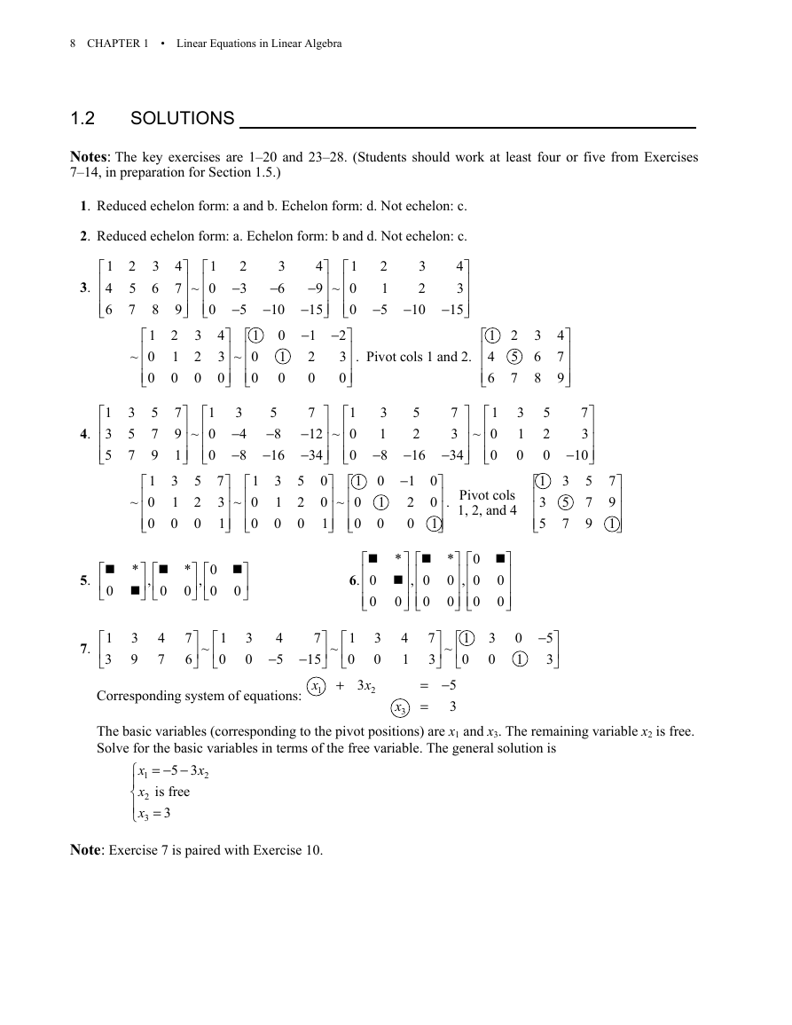
1. Reduced echelon form: a and b. Echelon form: d. Not echelon: c.
2. Reduced echelon form: a. Echelon form: b and d. Not echelon: c.
3.
1
4
6
4.
1
3
5
5.
0
2
5
7
3
6
8
1
~ 0
0
3
5
7
5
7
9
1
~ 0
0
4
1
7 ~ 0
9
0
2
1
0
3
2
0
7
1
9 ~ 0
1
0
3
1
0
5
2
0
2
−
3
−
5
4
1
3 ~ 0
0
0
3
−
4
−
8
1
7
3 ~ 0
1
0
3
−
6
−
10
0
1
0
5
−
8
−
16
3
1
0
*
,
0
*
0
,
0
0
0
2
1
−
5
3
2
−
10
4
3
−
15
. Pivot cols 1 and 2.
4
1
−
9 ~ 0
−
15
0
−
−
2
1
2
3
0
0
1
4
6
2
5
7
7
1
−
12 ~ 0
−
0
34
0
1
0 ~ 0
1
0
5
2
0
3
1
−
8
0
1
0
5
2
−
16
−
1
2
0
7
1
3 ~ 0
−
34
0
3
1
0
0
0
1
. Pivot cols
1, 2, and 4
6.
0
0
*
0
, 0
0
*
0
0 , 0
0
0
0
0
3
6
8
5
2
0
1
3
5
4
7
9
7
3
−
10
5
7
9
3
5
7
7
9
1
7.
4
7
3
9
1
3
7
−
15
x
Corresponding system of equations: 1
4
−
5
1
0
3
0
7
6
~
1
0
~
+
3
0
3
x
2
4
1
x
3
1
0
3
0
0
1
−
5
3
~
7
3
= −
5
=
3
The basic variables (corresponding to the pivot positions) are x1 and x3. The remaining variable x2 is free.
Solve for the basic variables in terms of the free variable. The general solution is
x
1
x
2
x
3
= − −
5 3
is free
=
3
x
2
Note: Exercise 7 is paired with Exercise 10.
�



 2023年江西萍乡中考道德与法治真题及答案.doc
 2012年重庆南川中考生物真题及答案.doc
 2013年江西师范大学地理学综合及文艺理论基础考研真题.doc
 2020年四川甘孜小升初语文真题及答案I卷.doc
 2020年注册岩土工程师专业基础考试真题及答案.doc
 2023-2024学年福建省厦门市九年级上学期数学月考试题及答案.doc
 2021-2022学年辽宁省沈阳市大东区九年级上学期语文期末试题及答案.doc
 2022-2023学年北京东城区初三第一学期物理期末试卷及答案.doc
 2018上半年江西教师资格初中地理学科知识与教学能力真题及答案.doc
 2012年河北国家公务员申论考试真题及答案-省级.doc
 2020-2021学年江苏省扬州市江都区邵樊片九年级上学期数学第一次质量检测试题及答案.doc
 2022下半年黑龙江教师资格证中学综合素质真题及答案.doc