Principles of
Geographical
Information
Systems
Peter A. Burrough
AND
Rachael A. McDonnell
OXFORD UNIVERSITY PRESS
1998
�
Data Models and Axioms
TWO
Data Models and Axioms:
Formal Abstractions
of Reality
When someone views an environment they simplify the inherent
complexity of it by abstracting key features to create a 'model' of the
area. This cognitive exercise is influenced by the cultural norms of
the observer and the purpose of the study. This chapter examines
the various model development stages that take place in the
process of producing geographical data that may be used by others
in a graphical or digital form. It is important to examine these
theoretical ideas as all the data we use in a GIS will have been
schematized using these geographical data models.
The two extremes in approach perceive space either as being
occupied by a series of entities which are described by their
properties and mapped using a co- ordinate system, or as a
continuous field of variation with no distinct boundaries. Formalized
geographical data models are used
these
conceptual ideas so that they may be broken down into units which
may be recorded and mapped. The principal approaches use either
a series of points, lines, and polygons, or tessellated units to
describe the various features in a landscape. The adoption of a
particular model influences the type of data that may be used to
describe the phenomena and the spatial analysis that may be
undertaken. The fundamental procedures and axioms for handling
and modifying spatial data are explained. Practical examples of the
choice and use of various data models in frequently encountered
applications are given.
to characterize
Imagine that you are talking on the telephone to
someone and they ask you to describe the view
from your window. How would you depict the
variations you see? It is likely that you would
break down the landscape
into units such as a building, road, field,
valley, or hill and use geographical referencing in
terms of 'beside', 'to the left of', or 'in front of' to
describe the features. You have in fact developed
a conceptual model of the
17
�
Data Models and Axioms
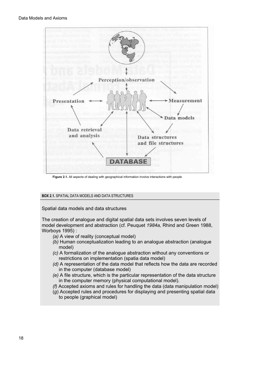
Figure 2.1. All aspects of dealing with geographical information involve interactions with people
BOX 2.1. SPATIAL DATA MODELS AND DATA STRUCTURES
Spatial data models and data structures
The creation of analogue and digital spatial data sets involves seven levels of
model development and abstraction (cf. Peuquet 1984a, Rhind and Green 1988,
Worboys 1995) :
(a) A view of reality (conceptual model)
(b) Human conceptualization leading to an analogue abstraction (analogue
model)
(c) A formalization of the analogue abstraction without any conventions or
restrictions on implementation (spatia data model)
(d) A representation of the data model that reflects how the data are recorded
in the computer (database model)
(e) A file structure, which is the particular representation of the data structure
in the computer memory (physical computational model).
(f) Accepted axioms and rules for handling the data (data manipulation model)
(g) Accepted rules and procedures for displaying and presenting spatial data
to people (graphical model)
18
�
these
remotely
sensed
landscape. Your interpretation of the features you
have observed and the ones you have decided to
ignore will be influenced by your experience, your
cultural background, and that of the person to
whom you are describing the scene.
Data Models and Axioms
world phenomena in the computer but only
representations based on
formalized
models. The major steps involved in proceeding
from human observation of the world, either
directly or with the assistance of tools like aerial
photographs,
images, or
statistically located samples, to an analogue or
digital representation are outlined in Box 2.1 and
illustrated in Figure 2.1. The most important first
step is that people observe the world and
perceive phenomena that are fixed or change in
space and time. Their perception will influence
all subsequent analysis; success or failure with
GIS does not depend in the first instance on
technology but more on the appropriateness or
otherwise of the conceptual models of space and
spatial interactions.
When information needs to be exchanged over a
larger domain it becomes necessary to formalize
the models used to describe an area to ensure that
data are
interpreted without ambiguity and
communicated effectively. This chapter will
describe the main data models used for describing
geographical phenomena (see Couclelis 1992,
Frank et al. 1992; Frank and Campari 1993;
Egenhofer and Herring 1995; and Burrough and
Frank 1996 for more detailed discussion). It gives
an essential background to the following chapters
of this book, because we do not store real
Conceptual models of real world geographical" phenomena
entation
structures.
Geographical phenomena require two descriptors
to represent the real world; what is present, and
Phenomena are also very often grouped or
where it is. For the former, phenomenological
divided into units at other levels of resolution
('scales') according to hierarchically defined
concepts such as
'floodplain',
taxonomies; for example
the hierarchy of
'ecotope', 'soil association' are used as fundamental
administration units of country-province-town-
building blocks for analysing and synthesizing
district, or of most soil, plant, or animal
complex
information. These phenomena are
classification systems.
recognized and described in terms of well-
established 'objects' or 'entities', which are de-
fined in standard texts (cf. Goudie et al. 1988,
Johnston et al. 1988, Lapedes 1976, Lapidus 1987,
Scott 1980, Stevens 1988, Whitten and Brooks
1972, Whittow 1984). However, these dictionaries
fail to point out that there are many ways to
describe these phenomena, and different terms can
be used for different levels of resolution. Many of
these
phenomena
described by people as explicit entities (such as
'hill', 'town', or 'lake') do not have an exact form
and their extent may change with time (e.g. see
Burrough and Frank 1996).
The referencing in space of the phenomena
may be defined in terms of a geometrically exact
or a relative location. The former uses local or
world coordinate systems defined using a
standard system of spheroids, projections, and
coordinates which give an approximation of the
form of the earth (a spheroid) onto a flat surface.
The coordinate system may be purely local,
measured in tens of metres, or it may be a
national grid or an internationally accepted
projection that uses geometrical coordinates of
latitude and longitude. Alternatively some maps
provide geographical referencing in a relative,
rather than an absolute spatial geometry as
illustrated by aboriginal rock paintings and the
plan of the London Underground. With these
maps the locations are defined in reference to
other features within the space, and neighbour-
hoodness and direction between entities is shown
rather than actual metric distances.
At the same time, the type of building block
used to describe a phenomena at one scale of
resolution is likely to be quite different from that
at another. For example, a road imaged from a
satellite-based sensor might be modelled as a line,
but the plan of a building site would have to be
modelled using an areal repres-
to
show
its various
'town',
'river',
perceived
geographical
19
�
it
is possible
to formalize
Data Models and Axioms
Conceptual models of space: entities or fields
Is the geographic world a jig-saw puzzle of
polygons. or a dub-sandwich of data layers?
(Coudelis 1992)
From these conceptual ideas of geographical
phenomena
the
representation of space and spatial properties.
When considering any space-a room, a landscape,
or
several
fundamentally different ways to describe what is
going on in that subset of the earth's surface. The
two extremes are (a) to perceive the space as being
occupied by entities which are described by their
attributes or properties, and whose position can be
mapped using a geometric coordinate system, or
(b) to imagine that the variation of an attribute of
interest varies over the space as some continuous
mathematical function or field.
-we may
continent
adopt
a
Entities. The most common view is that space
is peopled with 'objects' (entities). Defining and
recognizing the entity (is it a house, a cable, a
forest, a river, a mountain?) is the first step; listing
its attributes, defining its boundaries and its
location is the second. In this book we use the
word entity for those things that most people
would call an 'object' because the term 'object
orientation' has acquired a very special meaning in
database
(see
Chapter 3). In this jargon, 'object-orientation' is
used to refer to a way of structuring data in the
computer or in a computer program and does not
necessarily mean that a physical entity is being
referred to.
technology and programming
in
the
simplest
Continuous fields. In the continuous field
conceptual model
approach,
represents geographical space
terms of
continuous Cartesian coordinates in two or three
dimensions (or four if time is included). The
attribute is usually assumed to vary smoothly and
continuously over that space. The attribute (e.g. air
pressure, temperature, elevation above sea level,
clay content of the soil) and its spatial variation is
considered first; only when there are remarkable
clusters of like attribute values in geographical
space or time, as with hurricanes or mountain
peaks, or 'significant events' will these zones be
recognized as 'things' (e.g. Hurricane Caesar, the
Matterhorn, the Gulf Stream, or the clay layer rich
in the element
20
Indium that is thought to date the asteroid impact
that caused the demise of the dinosaurs).
Objects in a vector GIS may be counted,
moved about, stacked, rotated, colored,
labeled, cut, split, sliced, stuck together,
viewed from different angles, shaded, inflated,
shrunk, stored and retrieved, and in general,
handled like a variety of everyday solid
objects that bear no particular relationship to
geography. (Couclelis 1992)
the attribute
Opting for an entity model or a continuous
field approach can be difficult when the entities
can also be seen as sets of extreme attribute
values clustered in geographical space. Should
one recognize Switzerland, for example, as a
land of individual mountain entities (Mont
Blanc, Eiger, Matterhorn, etc.) or as a land in
which
'elevation' demonstrates
extreme variation? In practice, a pragmatic
solution based on the aims of the user of the
database must be made. The choice of
conceptual model determines how information
can later be derived. Opting for an entity
approach to mountain peaks will provide an
excellent basis for a system that records who
climbed the mountain and when, but it will not
provide information for computing the slopes of
its sides. Choosing a continuous representation
allows the calculation of slopes as the first
derivative of the surface, but does not give
names for those parts of the surface where the
first derivative is zero and the curvature is in
every direction downwards i.e. the peaks.
...the phenomenon of interest is blithely
bisected by the image frame. ..for the mindless
mechanical eye everything in the world is just
another array of pixels. (Couclelis 1992)
As a gross oversimplification, the choice of
an entity or a field approach also depends on the
scientific
�
Data Models and Axioms
Figure 2.2. Examples of the different kinds of geographical data collected for different purposes
by persons from different disciplines
or technical discipline of the observer. Disciplines
that focus on
the understanding of spatial
processes in the natural environment may be more
likely to use
the continuous field approach while those who
work entirely in an administrative context will
view an area as a series of distinct units (Figure
2.2).
Geographical data models and geographical data primitives
Geographical data models are the formalized
equivalents of the conceptual models used by
people to perceive geographical phenomena (in
this book we use the term 'data type' for the kind
of number used to quantify the attributes-see
below). They formalize how space is discretized
into parts for analysis and communication and
assume
that phenomena can be uniquely
identified, that attributes can be measured or
specified and that geographical coordinates can be
registered. As data may be collected in a variety of
ways,
information on the method or the level of
resolution of observation or measurement may
also be an important part of the data model.
agricultural
Most anthropogenic phenomena (houses, land
parcels, administrative units, roads, cables,
pipelines,
in Western
agriculture) can be handled best using the entity
approach. The simplest and most frequently used
data model of reality is a basic spatial entity
which is further specified by attributes and
geographical location. This can be further
fields
21
�
Data Models and Axioms
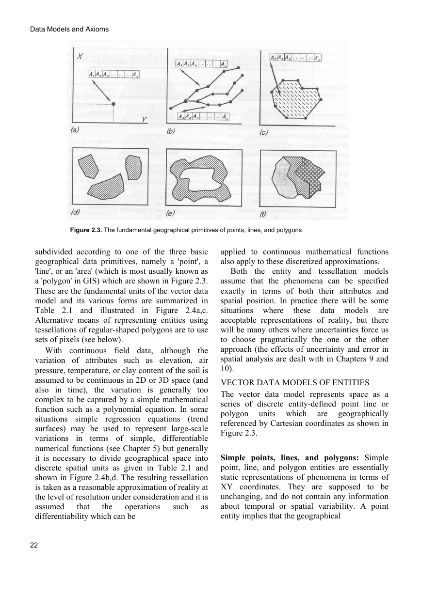
Figure 2.3. The fundamental geographical primitives of points, lines, and polygons
subdivided according to one of the three basic
geographical data primitives, namely a 'point', a
'line', or an 'area' (which is most usually known as
a 'polygon' in GIS) which are shown in Figure 2.3.
These are the fundamental units of the vector data
model and its various forms are summarized in
Table 2.1 and
in Figure 2.4a,c.
Alternative means of representing entities using
tessellations of regular-shaped polygons are to use
sets of pixels (see below).
illustrated
With continuous field data, although
the
variation of attributes such as elevation, air
pressure, temperature, or clay content of the soil is
assumed to be continuous in 2D or 3D space (and
also in time), the variation is generally too
complex to be captured by a simple mathematical
function such as a polynomial equation. In some
situations simple regression equations (trend
surfaces) may be used to represent large-scale
variations
terms of simple, differentiable
numerical functions (see Chapter 5) but generally
it is necessary to divide geographical space into
discrete spatial units as given in Table 2.1 and
shown in Figure 2.4b,d. The resulting tessellation
is taken as a reasonable approximation of reality at
the level of resolution under consideration and it is
assumed
as
differentiability which can be
operations
such
in
that
the
Both
applied to continuous mathematical functions
also apply to these discretized approximations.
the entity and
tessellation models
assume that the phenomena can be specified
exactly in terms of both their attributes and
spatial position. In practice there will be some
situations where
these data models are
acceptable representations of reality, but there
will be many others where uncertainties force us
to choose pragmatically the one or the other
approach (the effects of uncertainty and error in
spatial analysis are dealt with in Chapters 9 and
10).
VECTOR DATA MODELS OF ENTITIES
The vector data model represents space as a
series of discrete entity-defined point line or
polygon units which
are geographically
referenced by Cartesian coordinates as shown in
Figure 2.3.
Simple points, lines, and polygons: Simple
point, line, and polygon entities are essentially
static representations of phenomena in terms of
XY coordinates. They are supposed to be
unchanging, and do not contain any information
about temporal or spatial variability. A point
entity implies that the geographical
22
�
Data Models and Axioms
Tabble 2.1 Discrete data models for spatial data
Vector representation of exact entities
Tessellations of continuous fields
Non-topological structures (loose points and lines
“spaghetti”)
Regular triangular, square, or hexagonal
grid (square pixels = raster)
Simple topology with linked lines – e.g. a
drainage net or utility infrastrutures
Complex topology with linked lines and nest
structures – e.g linked polygons
Irregular tesselation: Thiessen polygons
Triangular irregular nets (TIN)
Finite elements
Complex topology of object orientation with
internal structures and relations.
Nested regular cells/quadtrees irregular
nesting
Figure 2.4. The encoding of exact objects (entities) and continuous fields in different data
models. (a) top left: vector representation of crisp polygons; (b) top right-raster model of
continuous fields; (c) bottom left-vector representation of linked lines; (d) bottom right-
Delaunay triangulation of a continuous field
23
�




 2023年江西萍乡中考道德与法治真题及答案.doc
 2012年重庆南川中考生物真题及答案.doc
 2013年江西师范大学地理学综合及文艺理论基础考研真题.doc
 2020年四川甘孜小升初语文真题及答案I卷.doc
 2020年注册岩土工程师专业基础考试真题及答案.doc
 2023-2024学年福建省厦门市九年级上学期数学月考试题及答案.doc
 2021-2022学年辽宁省沈阳市大东区九年级上学期语文期末试题及答案.doc
 2022-2023学年北京东城区初三第一学期物理期末试卷及答案.doc
 2018上半年江西教师资格初中地理学科知识与教学能力真题及答案.doc
 2012年河北国家公务员申论考试真题及答案-省级.doc
 2020-2021学年江苏省扬州市江都区邵樊片九年级上学期数学第一次质量检测试题及答案.doc
 2022下半年黑龙江教师资格证中学综合素质真题及答案.doc