Journal of Power and Energy Engineering, 2017, 5, 30-44
http://www.scirp.org/journal/jpee
ISSN Online: 2327-5901
ISSN Print: 2327-588X
Matlab Code to Assess the Reliability of the
Smart Power Distribution System
Using Monte Carlo Simulation
Tawfiq M. Aljohani1, Mohammed J. Beshir2
1Department of Electrical Engineering, Taibah University, Medina, KSA
2University of Southern California, Los Angeles, California, USA
How to cite this paper: Aljohani, T.M. and
Beshir, M.J. (2017) Matlab Code to Assess
the Reliability of the Smart Power Distribu-
tion System Using Monte Carlo Simulation.
Journal of Power and Energy Engineering,
5, 30-44.
https://doi.org/10.4236/jpee.2017.58003
Received: June 8, 2017
Accepted: August 7, 2017
Published: August 10, 2017
Copyright © 2017 by authors and
Scientific Research Publishing Inc.
This work is licensed under the Creative
Commons Attribution International
License (CC BY 4.0).
http://creativecommons.org/licenses/by/4.0/
Open Access
Abstract
Reliability of power systems is a key aspect in modern power system planning,
design, and operation. The ascendance of the smart grid concept has provided
high hopes of developing an intelligent network that is capable of being a
self-healing grid, offering the ability to overcome the interruption problems
that face the utility and cost it tens of millions in repair and loss. In this work,
we develop a MATLAB code to examine the effect of the smart grid applica-
tions in improving the reliability of the power distribution networks via
Monte Carlo Simulation approach. The system used in this paper is the IEEE
34 test feeder. The objective is to measure the installations of the Automatic
Reclosers (ARs) as well as the Distributed Generators (DGs) on the reliability
indices, SAIDI, SAIFI, CAIDI and EUE, and make comparisons with results
from a previous study done by the authors using another approach. The
MATLAB code should provide close results to the output of the previous re-
search to verify its effectiveness.
Keywords
Monte Carlo Simulation, Matlab Code for Power Systems Reliability, Power
System Reliability, Distributed Generators, Auto Reclosers, Reliability Indices,
Smart Grid
1. Introduction
The application of Monte Carlo simulation (MCS) is a corner-stone in the sensi-
tivity and quantitative probabilistic analysis. Among many of its great virtues is
its powerful ability to accurately evaluate the reliability of the electrical grid,
DOI: 10.4236/jpee.2017.58003 Aug. 10, 2017
30
Journal of Power and Energy Engineering
�
T.M. Aljohani, M. J. Beshir
which allowed several studies to emerge in this arena. The deterministic ap-
proach in assessing the reliability of the power systems is criticized for not being
sensitive to the stochastic nature of the grid as well as to customer demands and
components failures, which may lead to either an overinvestment or catastrophic
consequences. Therefore, the need for probabilistic evaluation of the electrical
system behavior has been emphasized in the most recent decade. MCS, as a
process of simulation, is strictly random and can be divided into two main types;
sequential and non-sequential (random) Monte Carlo methods. The sequential
MCS simulates the system operation as an up-and-down, where a system oper-
ating cycle is obtained by combining all the cycles of the system components in
chronological order. This usually requires more computational efforts than the
other approach, the non-sequential MCS, which simulates the system with a
higher efficiency by choosing intervals randomly, yet cannot simulate the chro-
nological aspect of the system behavior. The MCS process is central in the sto-
chastic simulation using random variables, where it can simulate the electrical
components considering the grid’s behavior with the goal of evaluating its ex-
pected reliability parameters [1] [2]. It also provides distribution information for
the load point indices, system indices, and the energy not served costs [3] [4].
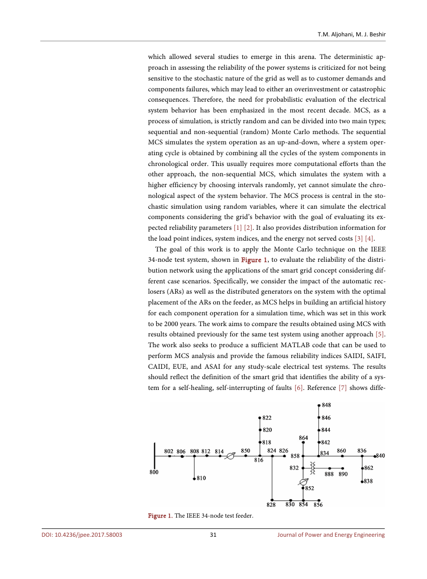
The goal of this work is to apply the Monte Carlo technique on the IEEE
34-node test system, shown in Figure 1, to evaluate the reliability of the distri-
bution network using the applications of the smart grid concept considering dif-
ferent case scenarios. Specifically, we consider the impact of the automatic rec-
losers (ARs) as well as the distributed generators on the system with the optimal
placement of the ARs on the feeder, as MCS helps in building an artificial history
for each component operation for a simulation time, which was set in this work
to be 2000 years. The work aims to compare the results obtained using MCS with
results obtained previously for the same test system using another approach [5].
The work also seeks to produce a sufficient MATLAB code that can be used to
perform MCS analysis and provide the famous reliability indices SAIDI, SAIFI,
CAIDI, EUE, and ASAI for any study-scale electrical test systems. The results
should reflect the definition of the smart grid that identifies the ability of a sys-
tem for a self-healing, self-interrupting of faults [6]. Reference [7] shows diffe-
DOI: 10.4236/jpee.2017.58003
Figure 1. The IEEE 34-node test feeder.
31
Journal of Power and Energy Engineering
�
T.M. Aljohani, M. J. Beshir
rent emerging technologies of the auto-reclosers that are now available in the
industry.
2. Monte Carlo Study
2.1. Concept of MCS
A Monte Carlo Simulation’s Matlab code was developed at the University of
Southern California by the authors of this paper to achieve the purpose of this
study. The code can be found in Appendix of this work. The input data utilized
in this work represents a real system data taken from reference [1], which was
also used in the reliability study done by the authors in [5]. The distribution sys-
tem reliability in overall is evaluated using load point indices and system indices,
which are the average failure rate (λi), average outage time (r), and the average
annual unavailability (U). The method considered in the coding is the time-se-
quential MCS, which models the system recognizing the chronological order as
the incidents occur on the system through the simulation time. An artificial his-
tory is generated using the random number generator which produces a uniform
random number (between 0 and 1) for each component in the test system for the
goal of providing a sequence of the operating-repairing cycle for it.
ln
TTF
i
= −
TTR
i
= −
ln
×
8760 hours
)
i
(
U
λ
i
(
U MTTR
i
×
)
i
hours
We simulated the IEEE test system using the famous two-state Markov model
shown in Figure 2 for all the non-source components in the feeder. The process
is highly random in nature as we do not know for sure when, where and which
component in the system will fail first with the fact that the behavior will be dif-
ferent from one component to another, including the type and number of fail-
ures as well as the time between a failure and restoration of a component. This
fact contributes to the virtue of MCS as a powerful tool to model these real be-
havior patterns in a simulated time for the sake of producing average reliability
values for a system when considering major design changes, such the integration
of smart grid technologies in its infrastructure. The Markov model has two
states; either up which for the operating condition of the components, or down
for the failing state. The up-state is also referred as TTF (time-to-fail) while the
down-state referred as TTR (time-to-repair/replace). It is noted that both TTR
and TTF are random in nature. The process from up to down is known as the
DOI: 10.4236/jpee.2017.58003
Figure 2. The two-state model of a component.
32
Journal of Power and Energy Engineering
�
T.M. Aljohani, M. J. Beshir
failure process for a component due to contingency event that would take it out
of operation. MCS randomly sample the up and down states for each element in
the feeder which generates a simulated sequence for the component’s history of
operation and failure. This helps in producing an overall conclusion about the
system behavior in general, and to identify the component that is prone to out-
ages in particular. Figure 3 illustrates the concept of TTR and TTF for a com-
ponent in any system. These times can be represented by random variables and
simulated using gamma, exponential, normal, lognormal and Poisson distribu-
tions [7] [8].
2.2. MCS Simulation Process
References [2] [6] [9] provided guidance on the MCS process that was utilized in
this work. The process can be simply briefed as follow:
1) Generate a random value for each of the component using the random num-
ber generator. The variable obtained for each component take the value be-
tween (0, 1) with equal likelihood.
2) Determine the component in the grid with the minimum TTF.
3) Convert the generated values into TTF, TTR for each component in the sys-
tem. Determine the outage duration for each failed load point indices.
4) Generate a new random number for the failed component and convert it into
a new TTF. If the simulation time is less than a year then return to step 2.
Otherwise, go to step 7.
5) Calculate the number and duration of failures for each load point per year.
6) Calculate the average value of the load point failure rate and duration for the
sample years.
7) Calculate SAIDI, SAIFI and system indices and record the average values of
the results.
8) Return to step 2 if the simulation time is less than the specified total simula-
tion years. Otherwise, record the results as final outcomes and end the simula-
tion.
3. Modeling the Test System in Matlab Considering
Smart Grid Technologies
3.1. Case 1(A): Installation of One Automatic Recloser
(AR) in the Feeder
The results of modeling the test system in our MATLAB code are provided in
Table 1. The application of the smart grid technologies on the reliability of the
DOI: 10.4236/jpee.2017.58003
Figure 3. The operating/failure time of a component.
33
Journal of Power and Energy Engineering
�
T.M. Aljohani, M. J. Beshir
DOI: 10.4236/jpee.2017.58003
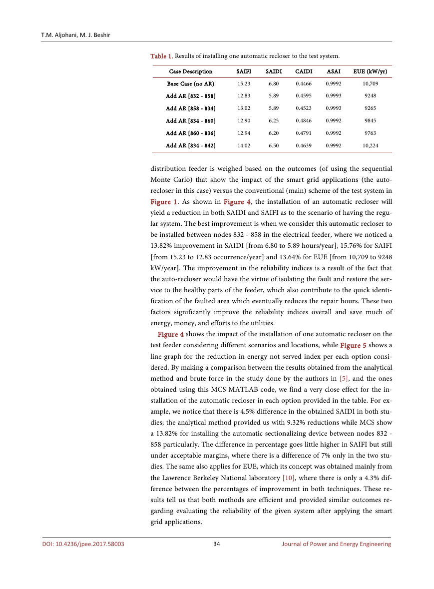
Table 1. Results of installing one automatic recloser to the test system.
Case Description
SAIFI
SAIDI
CAIDI
Base Case (no AR)
Add AR [832 - 858]
Add AR [858 - 834]
Add AR [834 - 860]
Add AR [860 - 836]
Add AR [834 - 842]
15.23
12.83
13.02
12.90
12.94
14.02
6.80
5.89
5.89
6.25
6.20
6.50
0.4466
0.4595
0.4523
0.4846
0.4791
0.4639
ASAI
0.9992
0.9993
0.9993
0.9992
0.9992
0.9992
EUE (kW/yr)
10,709
9248
9265
9845
9763
10,224
distribution feeder is weighed based on the outcomes (of using the sequential
Monte Carlo) that show the impact of the smart grid applications (the auto-
recloser in this case) versus the conventional (main) scheme of the test system in
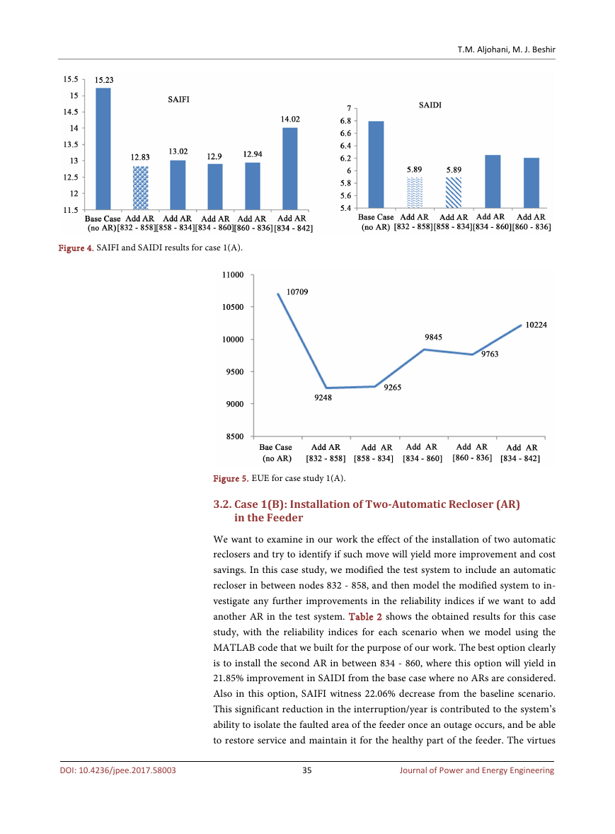
Figure 1. As shown in Figure 4, the installation of an automatic recloser will
yield a reduction in both SAIDI and SAIFI as to the scenario of having the regu-
lar system. The best improvement is when we consider this automatic recloser to
be installed between nodes 832 - 858 in the electrical feeder, where we noticed a
13.82% improvement in SAIDI [from 6.80 to 5.89 hours/year], 15.76% for SAIFI
[from 15.23 to 12.83 occurrence/year] and 13.64% for EUE [from 10,709 to 9248
kW/year]. The improvement in the reliability indices is a result of the fact that
the auto-recloser would have the virtue of isolating the fault and restore the ser-
vice to the healthy parts of the feeder, which also contribute to the quick identi-
fication of the faulted area which eventually reduces the repair hours. These two
factors significantly improve the reliability indices overall and save much of
energy, money, and efforts to the utilities.
Figure 4 shows the impact of the installation of one automatic recloser on the
test feeder considering different scenarios and locations, while Figure 5 shows a
line graph for the reduction in energy not served index per each option consi-
dered. By making a comparison between the results obtained from the analytical
method and brute force in the study done by the authors in [5], and the ones
obtained using this MCS MATLAB code, we find a very close effect for the in-
stallation of the automatic recloser in each option provided in the table. For ex-
ample, we notice that there is 4.5% difference in the obtained SAIDI in both stu-
dies; the analytical method provided us with 9.32% reductions while MCS show
a 13.82% for installing the automatic sectionalizing device between nodes 832 -
858 particularly. The difference in percentage goes little higher in SAIFI but still
under acceptable margins, where there is a difference of 7% only in the two stu-
dies. The same also applies for EUE, which its concept was obtained mainly from
the Lawrence Berkeley National laboratory [10], where there is only a 4.3% dif-
ference between the percentages of improvement in both techniques. These re-
sults tell us that both methods are efficient and provided similar outcomes re-
garding evaluating the reliability of the given system after applying the smart
grid applications.
34
Journal of Power and Energy Engineering
�
Figure 4. SAIFI and SAIDI results for case 1(A).
T.M. Aljohani, M. J. Beshir
Figure 5. EUE for case study 1(A).
3.2. Case 1(B): Installation of Two-Automatic Recloser (AR)
in the Feeder
We want to examine in our work the effect of the installation of two automatic
reclosers and try to identify if such move will yield more improvement and cost
savings. In this case study, we modified the test system to include an automatic
recloser in between nodes 832 - 858, and then model the modified system to in-
vestigate any further improvements in the reliability indices if we want to add
another AR in the test system. Table 2 shows the obtained results for this case
study, with the reliability indices for each scenario when we model using the
MATLAB code that we built for the purpose of our work. The best option clearly
is to install the second AR in between 834 - 860, where this option will yield in
21.85% improvement in SAIDI from the base case where no ARs are considered.
Also in this option, SAIFI witness 22.06% decrease from the baseline scenario.
This significant reduction in the interruption/year is contributed to the system’s
ability to isolate the faulted area of the feeder once an outage occurs, and be able
to restore service and maintain it for the healthy part of the feeder. The virtues
35
Journal of Power and Energy Engineering
DOI: 10.4236/jpee.2017.58003
�
T.M. Aljohani, M. J. Beshir
DOI: 10.4236/jpee.2017.58003
Table 2. The results of modeling the test system with two ARs.
Case Description
SAIFI
SAIDI
CAIDI
EUE (kW)
Add AR [834 - 860]
Add AR [860 - 836]
Add AR [834 - 842]
Add AR [832 - 888]
Add AR [842 - 844]
11.87
12.30
12.18
12.76
12.61
5.314
5.541
5.450
5.79
5.64
0.4474
0.4504
0.4472
0.4587
0.4476
8361
8707
8565
9065
8869
of modeling the system using MCS is its ability to offer the best location for the
ARs considering the artificial data it made for each component of up and down
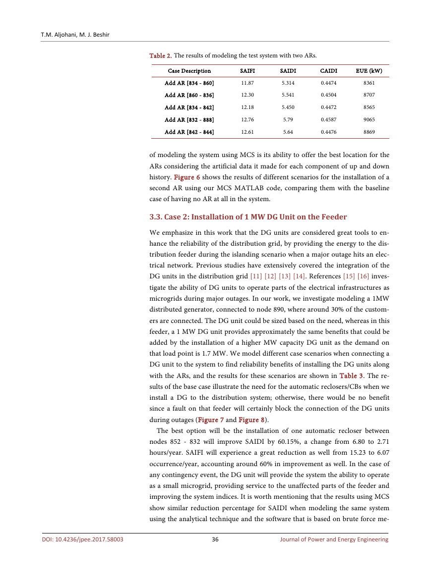
history. Figure 6 shows the results of different scenarios for the installation of a
second AR using our MCS MATLAB code, comparing them with the baseline
case of having no AR at all in the system.
3.3. Case 2: Installation of 1 MW DG Unit on the Feeder
We emphasize in this work that the DG units are considered great tools to en-
hance the reliability of the distribution grid, by providing the energy to the dis-
tribution feeder during the islanding scenario when a major outage hits an elec-
trical network. Previous studies have extensively covered the integration of the
DG units in the distribution grid [11] [12] [13] [14]. References [15] [16] inves-
tigate the ability of DG units to operate parts of the electrical infrastructures as
microgrids during major outages. In our work, we investigate modeling a 1MW
distributed generator, connected to node 890, where around 30% of the custom-
ers are connected. The DG unit could be sized based on the need, whereas in this
feeder, a 1 MW DG unit provides approximately the same benefits that could be
added by the installation of a higher MW capacity DG unit as the demand on
that load point is 1.7 MW. We model different case scenarios when connecting a
DG unit to the system to find reliability benefits of installing the DG units along
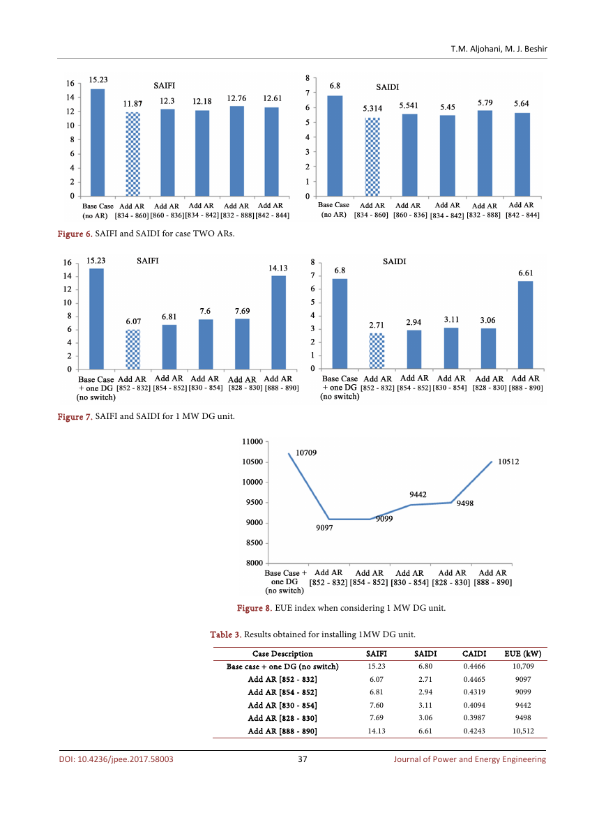
with the ARs, and the results for these scenarios are shown in Table 3. The re-
sults of the base case illustrate the need for the automatic reclosers/CBs when we
install a DG to the distribution system; otherwise, there would be no benefit
since a fault on that feeder will certainly block the connection of the DG units
during outages (Figure 7 and Figure 8).
The best option will be the installation of one automatic recloser between
nodes 852 - 832 will improve SAIDI by 60.15%, a change from 6.80 to 2.71
hours/year. SAIFI will experience a great reduction as well from 15.23 to 6.07
occurrence/year, accounting around 60% in improvement as well. In the case of
any contingency event, the DG unit will provide the system the ability to operate
as a small microgrid, providing service to the unaffected parts of the feeder and
improving the system indices. It is worth mentioning that the results using MCS
show similar reduction percentage for SAIDI when modeling the same system
using the analytical technique and the software that is based on brute force me-
36
Journal of Power and Energy Engineering
�
Figure 6. SAIFI and SAIDI for case TWO ARs.
Figure 7. SAIFI and SAIDI for 1 MW DG unit.
T.M. Aljohani, M. J. Beshir
Figure 8. EUE index when considering 1 MW DG unit.
Table 3. Results obtained for installing 1MW DG unit.
Case Description
Base case + one DG (no switch)
Add AR [852 - 832]
Add AR [854 - 852]
Add AR [830 - 854]
Add AR [828 - 830]
Add AR [888 - 890]
SAIFI
15.23
6.07
6.81
7.60
7.69
14.13
SAIDI
6.80
2.71
2.94
3.11
3.06
6.61
CAIDI
0.4466
0.4465
0.4319
0.4094
0.3987
0.4243
EUE (kW)
10,709
9097
9099
9442
9498
10,512
37
Journal of Power and Energy Engineering
DOI: 10.4236/jpee.2017.58003
�




 2023年江西萍乡中考道德与法治真题及答案.doc
 2012年重庆南川中考生物真题及答案.doc
 2013年江西师范大学地理学综合及文艺理论基础考研真题.doc
 2020年四川甘孜小升初语文真题及答案I卷.doc
 2020年注册岩土工程师专业基础考试真题及答案.doc
 2023-2024学年福建省厦门市九年级上学期数学月考试题及答案.doc
 2021-2022学年辽宁省沈阳市大东区九年级上学期语文期末试题及答案.doc
 2022-2023学年北京东城区初三第一学期物理期末试卷及答案.doc
 2018上半年江西教师资格初中地理学科知识与教学能力真题及答案.doc
 2012年河北国家公务员申论考试真题及答案-省级.doc
 2020-2021学年江苏省扬州市江都区邵樊片九年级上学期数学第一次质量检测试题及答案.doc
 2022下半年黑龙江教师资格证中学综合素质真题及答案.doc