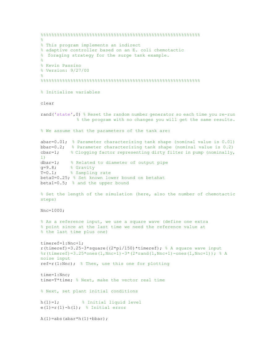
%%%%%%%%%%%%%%%%%%%%%%%%%%%%%%%%%%%%%%%%%%%%%%%%%%%%%%%%%%%
%
% This program implements an indirect
% adaptive controller based on an E. coli chemotactic
% foraging strategy for the surge tank example.
%
% Kevin Passino
% Version: 9/27/00
%
%%%%%%%%%%%%%%%%%%%%%%%%%%%%%%%%%%%%%%%%%%%%%%%%%%%%%%%%%%%
% Initialize variables
clear
rand('state',0) % Reset the random number generator so each time you re-run
% the program with no changes you will get the same results.
% We assume that the parameters of the tank are:
abar=0.01; % Parameter characterizing tank shape (nominal value is 0.01)
bbar=0.2;
% Parameter characterizing tank shape (nominal value is 0.2)
% Clogging factor representing dirty filter in pump (nominally,
cbar=1;
1)
% Related to diameter of output pipe
dbar=1;
g=9.8;
% Gravity
T=0.1;
% Sampling rate
beta0=0.25; % Set known lower bound on betahat
beta1=0.5; % and the upper bound
% Set the length of the simulation (here, also the number of chemotactic
steps)
Nnc=1000;
% As a reference input, we use a square wave (define one extra
% point since at the last time we need the reference value at
% the last time plus one)
timeref=1:Nnc+1;
r(timeref)=3.25-3*square((2*pi/150)*timeref); % A square wave input
%r(timeref)=3.25*ones(1,Nnc+1)-3*(2*rand(1,Nnc+1)-ones(1,Nnc+1)); % A
noise input
ref=r(1:Nnc); % Then, use this one for plotting
time=1:Nnc;
time=T*time; % Next, make the vector real time
% Next, set plant initial conditions
h(1)=1;
% Initial liquid level
e(1)=r(1)-h(1); % Initial error
A(1)=abs(abar*h(1)+bbar);
�
alpha(1)=h(1)-T*dbar*sqrt(2*g*h(1))/A(1);
beta(1)=T*cbar/A(1);
%%%%%%%%%%%%%%%%%%%%%%%%%%%%%%%%%%%%%%%
% Initialize the foraging strategy parameters:
%%%%%%%%%%%%%%%%%%%%%%%%%%%%%%%%%%%%%%%
% We will use a very simple foraging strategy, one modeling the E. coli,
but not
% the reproduction and elimination-dispersal events. We align the
increments for
% chemotactic steps with time steps (of course you could take multiple steps
per
% time step, but that complicates the coding a bit).
p=2;
S=10;
this to be an
% The number of bacteria in the population (for convenience, require
% an even number)
% Limits the length of a swim when it is on a gradient
% Dimension of the search space
Ns=4;
climbstepcounter=0*ones(S,1); % Set up a counter for each bacterium when
for how long it
% will climb down in a single direction
runlengthunit=0.05; % For setting chemotactic step size (same for both
dimensions), can
% think of this as an adaptation gain
Delta(:,i)=(2*round(rand(p,1))-1).*rand(p,1);
% Allocate memory:
%bestvalue=0*ones(Nnc+1,1);
%bestmember=0*ones(Nnc+1,1);
%bestindividual=0*ones(p,Nnc+1);
% Generate an initial random direction for each bacterium (later these will
change when
% a bacterium tumbles)
for i=1:S
end
% Initial population
P(:,:,:)=0*ones(p,S,Nnc+1); % First, allocate needed memory
% Initialize locations of bacteria - initial guess at the plant dynamics
(make each member of the
% population the same initial guess)
thetaalpha(1)=2;
�
thetabeta(1)=0.5;
for m=1:S
P(1,m,1)=thetaalpha(1); % Load into initial population of bacteria
P(2,m,1)=thetabeta(1);
end
% Make the initial estimates of the plant dynamics based on this:
alphahat(1)=thetaalpha(1)*h(1);
betahat(1)=thetabeta(1);
% Number of steps to look back in assessment of quality of identifier model:
N=100;
% Next, define the intial controller output
u(1)=(1/(betahat(1)))*(-alphahat(1)+r(1+1));
% Initialize estimate of the plant dynamics (note that the
% time indices are not properly aligned but this is just an estimate)
hhat(1)=alphahat(1)+betahat(1)*u(1); % Estimate to be the same as at
% the first time step
%%%%%%%%%%%%%%%%%%%%%%%%%%%%%
% Next, start the main loop:
%%%%%%%%%%%%%%%%%%%%%%%%%%%%%
for k=2:Nnc
% Define the plant
% In implementation, the input flow is restricted
% by some physical contraints. So we have to put a
% limit for the input flow that is chosen as 50.
if u(k-1)>50
u(k-1)=50;
end
if u(k-1)<-50
u(k-1)=-50;
end
h(k)=alpha(k-1)+beta(k-1)*u(k-1);
h(k)=max([0.001,h(k)]); % Constraint liquid not to go
% negative
e(k)=r(k)-h(k); % For plotting, if needed
% Define the adaptive controller:
�
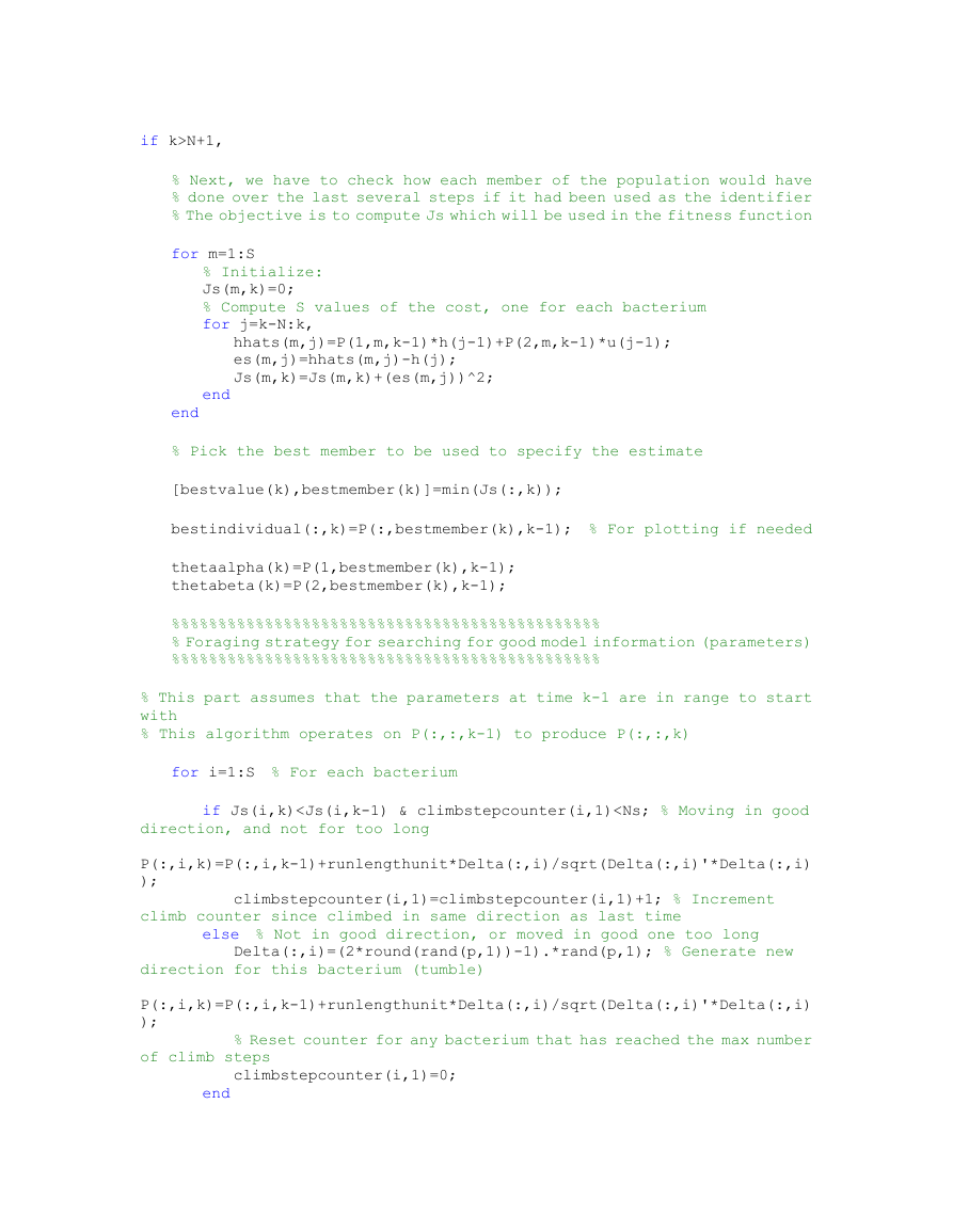
if k>N+1,
% Next, we have to check how each member of the population would have
% done over the last several steps if it had been used as the identifier
% The objective is to compute Js which will be used in the fitness function
for m=1:S
% Initialize:
Js(m,k)=0;
% Compute S values of the cost, one for each bacterium
for j=k-N:k,
hhats(m,j)=P(1,m,k-1)*h(j-1)+P(2,m,k-1)*u(j-1);
es(m,j)=hhats(m,j)-h(j);
Js(m,k)=Js(m,k)+(es(m,j))^2;
end
end
% Pick the best member to be used to specify the estimate
[bestvalue(k),bestmember(k)]=min(Js(:,k));
bestindividual(:,k)=P(:,bestmember(k),k-1); % For plotting if needed
thetaalpha(k)=P(1,bestmember(k),k-1);
thetabeta(k)=P(2,bestmember(k),k-1);
%%%%%%%%%%%%%%%%%%%%%%%%%%%%%%%%%%%%%%%%%%%%%%
% Foraging strategy for searching for good model information (parameters)
%%%%%%%%%%%%%%%%%%%%%%%%%%%%%%%%%%%%%%%%%%%%%%
% This part assumes that the parameters at time k-1 are in range to start
with
% This algorithm operates on P(:,:,k-1) to produce P(:,:,k)
for i=1:S % For each bacterium
if Js(i,k)
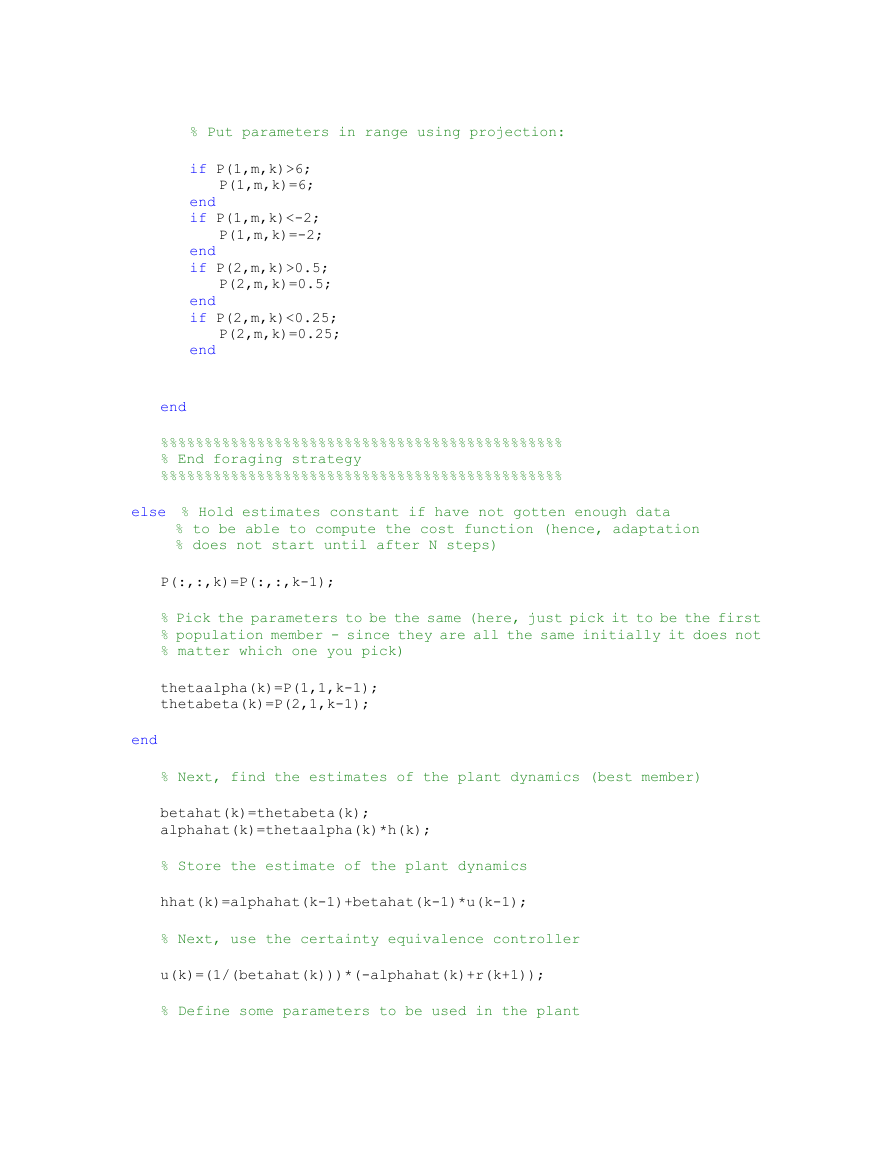
% Put parameters in range using projection:
if P(1,m,k)>6;
P(1,m,k)=6;
end
if P(1,m,k)<-2;
P(1,m,k)=-2;
end
if P(2,m,k)>0.5;
P(2,m,k)=0.5;
end
if P(2,m,k)<0.25;
P(2,m,k)=0.25;
end
end
%%%%%%%%%%%%%%%%%%%%%%%%%%%%%%%%%%%%%%%%%%%%%%
% End foraging strategy
%%%%%%%%%%%%%%%%%%%%%%%%%%%%%%%%%%%%%%%%%%%%%%
else % Hold estimates constant if have not gotten enough data
% to be able to compute the cost function (hence, adaptation
% does not start until after N steps)
P(:,:,k)=P(:,:,k-1);
% Pick the parameters to be the same (here, just pick it to be the first
% population member - since they are all the same initially it does not
% matter which one you pick)
thetaalpha(k)=P(1,1,k-1);
thetabeta(k)=P(2,1,k-1);
end
% Next, find the estimates of the plant dynamics (best member)
betahat(k)=thetabeta(k);
alphahat(k)=thetaalpha(k)*h(k);
% Store the estimate of the plant dynamics
hhat(k)=alphahat(k-1)+betahat(k-1)*u(k-1);
% Next, use the certainty equivalence controller
u(k)=(1/(betahat(k)))*(-alphahat(k)+r(k+1));
% Define some parameters to be used in the plant
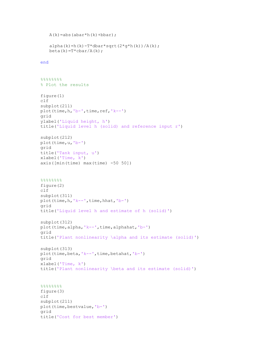
�
A(k)=abs(abar*h(k)+bbar);
alpha(k)=h(k)-T*dbar*sqrt(2*g*h(k))/A(k);
beta(k)=T*cbar/A(k);
end
%%%%%%%%
% Plot the results
figure(1)
clf
subplot(211)
plot(time,h,'b-',time,ref,'k--')
grid
ylabel('Liquid height, h')
title('Liquid level h (solid) and reference input r')
subplot(212)
plot(time,u,'b-')
grid
title('Tank input, u')
xlabel('Time, k')
axis([min(time) max(time) -50 50])
%%%%%%%%
figure(2)
clf
subplot(311)
plot(time,h,'k--',time,hhat,'b-')
grid
title('Liquid level h and estimate of h (solid)')
subplot(312)
plot(time,alpha,'k--',time,alphahat,'b-')
grid
title('Plant nonlinearity \alpha and its estimate (solid)')
subplot(313)
plot(time,beta,'k--',time,betahat,'b-')
grid
xlabel('Time, k')
title('Plant nonlinearity \beta and its estimate (solid)')
%%%%%%%%
figure(3)
clf
subplot(211)
plot(time,bestvalue,'b-')
grid
title('Cost for best member')
�
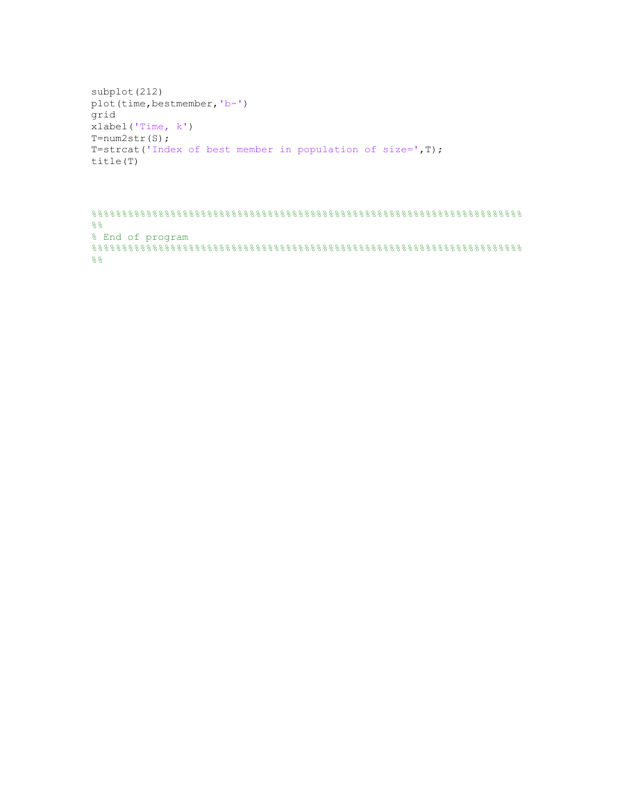
subplot(212)
plot(time,bestmember,'b-')
grid
xlabel('Time, k')
T=num2str(S);
T=strcat('Index of best member in population of size=',T);
title(T)
%%%%%%%%%%%%%%%%%%%%%%%%%%%%%%%%%%%%%%%%%%%%%%%%%%%%%%%%%%%%%%%%%%%%%%%
%%
% End of program
%%%%%%%%%%%%%%%%%%%%%%%%%%%%%%%%%%%%%%%%%%%%%%%%%%%%%%%%%%%%%%%%%%%%%%%
%%
�




 2023年江西萍乡中考道德与法治真题及答案.doc
 2012年重庆南川中考生物真题及答案.doc
 2013年江西师范大学地理学综合及文艺理论基础考研真题.doc
 2020年四川甘孜小升初语文真题及答案I卷.doc
 2020年注册岩土工程师专业基础考试真题及答案.doc
 2023-2024学年福建省厦门市九年级上学期数学月考试题及答案.doc
 2021-2022学年辽宁省沈阳市大东区九年级上学期语文期末试题及答案.doc
 2022-2023学年北京东城区初三第一学期物理期末试卷及答案.doc
 2018上半年江西教师资格初中地理学科知识与教学能力真题及答案.doc
 2012年河北国家公务员申论考试真题及答案-省级.doc
 2020-2021学年江苏省扬州市江都区邵樊片九年级上学期数学第一次质量检测试题及答案.doc
 2022下半年黑龙江教师资格证中学综合素质真题及答案.doc