Grey Wolf Optimizer（狼群算法最早的一篇文章）GWO.pdf

发布时间：2022-06-01 发布人：admin 分类：说明书资料大小：4.26M 资料格式：pdf 举报版权申诉

wq6qeg88-11184088-4744302542970957328.pdf-第1页.png

第1页 / 共16页

wq6qeg88-11184088-4744302542970957328.pdf-第2页.png

第2页 / 共16页

wq6qeg88-11184088-4744302542970957328.pdf-第3页.png

第3页 / 共16页

wq6qeg88-11184088-4744302542970957328.pdf-第4页.png

第4页 / 共16页

wq6qeg88-11184088-4744302542970957328.pdf-第5页.png

第5页 / 共16页

wq6qeg88-11184088-4744302542970957328.pdf-第6页.png

第6页 / 共16页

wq6qeg88-11184088-4744302542970957328.pdf-第7页.png

第7页 / 共16页

wq6qeg88-11184088-4744302542970957328.pdf-第8页.png

第8页 / 共16页

Grey Wolf Optimizer

1 Introduction

2 Literature review

3 Grey Wolf Optimizer (GWO)

3.1 Inspiration

3.2 Mathematical model and algorithm

3.2.1 Social hierarchy

3.2.2 Encircling prey

3.2.3 Hunting

3.2.4 Attacking prey (exploitation)

3.2.5 Search for prey (exploration)

4 Results and discussion

4.1 Exploitation analysis

4.2 Exploration analysis

4.3 Local minima avoidance

4.4 Convergence behavior analysis

5 GWO for classical engineering problems

5.1 Tension/compression spring design

5.2 Welded beam design

5.3 Pressure vessel design

6 Real application of GWO in optical engineering (optical buffer design)

7 Conclusion

Appendix A Supplementary material

References

Advances in Engineering Software 69 (2014) 46–61 Contents lists available at ScienceDirect Advances in Engineering Software j o u r n a l h o m e p a g e : w w w . e l s e v i e r . c o m / l o c a t e / a d v e n g s o f t Grey Wolf Optimizer Seyedali Mirjalili a,⇑ , Seyed Mohammad Mirjalili b, Andrew Lewis a a School of Information and Communication Technology, Grifﬁth University, Nathan Campus, Brisbane QLD 4111, Australia b Department of Electrical Engineering, Faculty of Electrical and Computer Engineering, Shahid Beheshti University, G.C. 1983963113, Tehran, Iran a r t i c l e i n f o a b s t r a c t Article history: Received 27 June 2013 Received in revised form 18 October 2013 Accepted 11 December 2013 Available online 21 January 2014 Keywords: Optimization Optimization techniques Heuristic algorithm Metaheuristics Constrained optimization GWO 1. Introduction This work proposes a new meta-heuristic called Grey Wolf Optimizer (GWO) inspired by grey wolves (Canis lupus). The GWO algorithm mimics the leadership hierarchy and hunting mechanism of grey wolves in nature. Four types of grey wolves such as alpha, beta, delta, and omega are employed for sim- ulating the leadership hierarchy. In addition, the three main steps of hunting, searching for prey, encir- cling prey, and attacking prey, are implemented. The algorithm is then benchmarked on 29 well-known test functions, and the results are veriﬁed by a comparative study with Particle Swarm Optimization (PSO), Gravitational Search Algorithm (GSA), Differential Evolution (DE), Evolutionary Programming (EP), and Evolution Strategy (ES). The results show that the GWO algorithm is able to provide very com- petitive results compared to these well-known meta-heuristics. The paper also considers solving three classical engineering design problems (tension/compression spring, welded beam, and pressure vessel designs) and presents a real application of the proposed method in the ﬁeld of optical engineering. The results of the classical engineering design problems and real application prove that the proposed algo- rithm is applicable to challenging problems with unknown search spaces. Ó 2013 Elsevier Ltd. All rights reserved. Meta-heuristic optimization techniques have become very pop- ular over the last two decades. Surprisingly, some of them such as Genetic Algorithm (GA) [1], Ant Colony Optimization (ACO) [2], and Particle Swarm Optimization (PSO) [3] are fairly well-known among not only computer scientists but also scientists from differ- ent ﬁelds. In addition to the huge number of theoretical works, such optimization techniques have been applied in various ﬁelds of study. There is a question here as to why meta-heuristics have become remarkably common. The answer to this question can be summarized into four main reasons: simplicity, ﬂexibility, deriva- tion-free mechanism, and local optima avoidance. First, meta-heuristics are fairly simple. They have been mostly inspired by very simple concepts. The inspirations are typically re- lated to physical phenomena, animals’ behaviors, or evolutionary concepts. The simplicity allows computer scientists to simulate dif- ferent natural concepts, propose new meta-heuristics, hybridize two or more meta-heuristics, or improve the current meta-heuris- tics. Moreover, the simplicity assists other scientists to learn meta- heuristics quickly and apply them to their problems. Second, ﬂexibility refers to the applicability of meta-heuristics to different problems without any special changes in the structure of the algorithm. Meta-heuristics are readily applicable to different ⇑ Corresponding author. Tel.: +61 434555738. E-mail addresses: seyedali.mirjalili@grifﬁthuni.edu.au (S. Mirjalili), mohammad.smm@gmail.com (S.M. Mirjalili), a.lewis@grifﬁth.edu.au (A. Lewis). 0965-9978/$ - see front matter Ó 2013 Elsevier Ltd. All rights reserved. http://dx.doi.org/10.1016/j.advengsoft.2013.12.007 problems since they mostly assume problems as black boxes. In other words, only the input(s) and output(s) of a system are impor- tant for a meta-heuristic. So, all a designer needs is to know how to represent his/her problem for meta-heuristics. In contrast Third, the majority of meta-heuristics have derivation-free mechanisms. to gradient-based optimization ap- proaches, meta-heuristics optimize problems stochastically. The optimization process starts with random solution(s), and there is no need to calculate the derivative of search spaces to ﬁnd the opti- mum. This makes meta-heuristics highly suitable for real problems with expensive or unknown derivative information. Finally, meta-heuristics have superior abilities to avoid local op- tima compared to conventional optimization techniques. This is due to the stochastic nature of meta-heuristics which allow them to avoid stagnation in local solutions and search the entire search space extensively. The search space of real problems is usually un- known and very complex with a massive number of local optima, so meta-heuristics are good options for optimizing these challeng- ing real problems. The No Free Lunch (NFL) theorem [4] is worth mentioning here. This theorem has logically proved that there is no meta-heuristic best suited for solving all optimization problems. In other words, a particular meta-heuristic may show very promising results on a set of problems, but the same algorithm may show poor perfor- mance on a different set of problems. Obviously, NFL makes this ﬁeld of study highly active which results in enhancing current ap- proaches and proposing new meta-heuristics every year. This also

S. Mirjalili et al. / Advances in Engineering Software 69 (2014) 46–61 47 motivates our attempts to develop a new meta-heuristic with inspiration from grey wolves. Generally speaking, meta-heuristics can be divided into two main classes: single-solution-based and population-based. In the former class (Simulated Annealing [5] for instance) the search pro- cess starts with one candidate solution. This single candidate solu- tion is then improved over the course of iterations. Population- based meta-heuristics, however, perform the optimization using a set of solutions (population). In this case the search process starts with a random initial population (multiple solutions), and this population is enhanced over the course of iterations. Population- based meta-heuristics have some advantages compared to single solution-based algorithms: Multiple candidate solutions share information about the search space which results in sudden jumps toward the prom- ising part of search space. Multiple candidate solutions assist each other to avoid locally optimal solutions. Population-based meta-heuristics generally have greater explo- ration compared to single solution-based algorithms. One of the interesting branches of the population-based meta- heuristics is Swarm Intelligence (SI). The concepts of SI was ﬁrst proposed in 1993 [6]. According to Bonabeau et al. [1], SI is ‘‘The emergent collective intelligence of groups of simple agents’’. The inspi- rations of SI techniques originate mostly from natural colonies, ﬂock, herds, and schools. Some of the most popular SI techniques are ACO [2], PSO [3], and Artiﬁcial Bee Colony (ABC) [7]. A compre- hensive literature review of the SI algorithms is provided in the next section. Some of the advantages of SI algorithms are: SI algorithms preserve information about the search space over the course of iteration, whereas Evolutionary Algorithms (EA) discard the information of the previous generations. SI algorithms often utilize memory to save the best solution obtained so far. SI algorithms usually have fewer parameters to adjust. SI algorithms have less operators compared to evolutionary approaches (crossover, mutation, elitism, and so on). SI algorithms are easy to implement. Regardless of the differences between the meta-heuristics, a common feature is the division of the search process into two phases: exploration and exploitation [8–12]. The exploration phase refers to the process of investigating the promising area(s) of the search space as broadly as possible. An algorithm needs to have sto- chastic operators to randomly and globally search the search space in order to support this phase. However, exploitation refers to the lo- cal search capability around the promising regions obtained in the exploration phase. Finding a proper balance between these two phases is considered a challenging task due to the stochastic nature of meta-heuristics. This work proposes a new SI technique with inspiration from the social hierarchy and hunting behavior of grey wolf packs. The rest of the paper is organized as follows: Section 2 presents a literature review of SI techniques. Section 3 outlines the proposed GWO algorithm. The results and discussion of benchmark functions, semi-real problems, and a real application are presented in Sections 4-6, respectively. Finally, Section 7 con- cludes the work and suggests some directions for future studies. 2. Literature review Meta-heuristics may be classiﬁed into three main classes: evolutionary, physics-based, and SI algorithms. EAs are usually inspired by the concepts of evolution in nature. The most popular algorithm in this branch is GA. This algorithm was proposed by Holland in 1992 [13] and simulates Darwnian evolution concepts. The engineering applications of GA were extensively investigated by Goldberg [14]. Generally speaking, the optimization is done by evolving an initial random solution in EAs. Each new population is created by the combination and mutation of the individuals in the previous generation. Since the best individuals have higher probability of participating in generating the new population, the new population is likely to be better than the previous genera- tion(s). This can guarantee that the initial random population is optimized over the course of generations. Some of the EAs are Dif- ferential Evolution (DE) [15], Evolutionary Programing (EP) [16,17], and Evolution Strategy (ES) [18,19], Genetic Programming (GP) [20], and Biogeography-Based Optimizer (BBO) [21]. As an example, the BBO algorithm was ﬁrst proposed by Simon in 2008 [21]. The basic idea of this algorithm has been inspired by biogeography which refers to the study of biological organisms in terms of geographical distribution (over time and space). The case studies might include different islands, lands, or even continents over decades, centuries, or millennia. In this ﬁeld of study different ecosystems (habitats or territories) are investigated for ﬁnding the relations between different species (habitants) in terms of immi- gration, emigration, and mutation. The evolution of ecosystems (considering different kinds of species such as predator and prey) over migration and mutation to reach a stable situation was the main inspiration of the BBO algorithm. The second main branch of meta-heuristics is physics-based techniques. Such optimization algorithms typically mimic physical rules. Some of the most popular algorithms are Gravitational Local Search (GLSA) [22], Big-Bang Big-Crunch (BBBC) [23], Gravitational Search Algorithm (GSA) [24], Charged System Search (CSS) [25], Central Force Optimization (CFO) [26], Artiﬁcial Chemical Reaction Optimization Algorithm (ACROA) [27], Black Hole (BH) [28] algo- rithm, Ray Optimization (RO) [29] algorithm, Small-World Optimi- zation Algorithm (SWOA) [30], Galaxy-based Search Algorithm (GbSA) [31], and Curved Space Optimization (CSO) [32]. The mech- anism of these algorithms is different from EAs, in that a random set of search agents communicate and move throughout search space according to physical rules. This movement is implemented, for example, using gravitational force, ray casting, electromagnetic force, inertia force, weights, and so on. For example, the BBBC algorithm was inspired by the big bang and big crunch theories. The search agents of BBBC are scattered from a point in random directions in a search space according to the principles of the big bang theory. They search randomly and then gather in a ﬁnal point (the best point obtained so far) accord- ing to the principles of the big crunch theory. GSA is another phys- ics-based algorithm. The basic physical theory from which GSA is inspired is Newton’s law of universal gravitation. The GSA algo- rithm performs search by employing a collection of agents that have masses proportional to the value of a ﬁtness function. During iteration, the masses are attracted to each other by the gravita- tional forces between them. The heavier the mass, the bigger the attractive force. Therefore, the heaviest mass, which is possibly close to the global optimum, attracts the other masses in propor- tion to their distances. The third subclass of meta-heuristics is the SI methods. These algorithms mostly mimic the social behavior of swarms, herds, ﬂocks, or schools of creatures in nature. The mechanism is almost similar to physics-based algorithm, but the search agents navigate using the simulated collective and social intelligence of creatures. The most popular SI technique is PSO. The PSO algorithm was pro- posed by Kennedy and Eberhart [3] and inspired from the social behavior of birds ﬂocking. The PSO algorithm employs multiple particles that chase the position of the best particle and their

48 S. Mirjalili et al. / Advances in Engineering Software 69 (2014) 46–61 own best positions obtained so far. In other words, a particle is moved considering its own best solution as well as the best solu- tion the swarm has obtained. Another popular SI algorithm is ACO, proposed by Dorigo et al. in 2006 [2]. This algorithm was inspired by the social behavior of ants in an ant colony. In fact, the social intelligence of ants in ﬁnd- ing the shortest path between the nest and a source of food is the main inspiration of ACO. A pheromone matrix is evolved over the course of iteration by the candidate solutions. The ABC is another popular algorithm, mimicking the collective behavior of bees in ﬁnding food sources. There are three types of bees in ABS: scout, onlooker, and employed bees. The scout bees are responsible for exploring the search space, whereas onlooker and employed bees exploit the promising solutions found by scout bees. Finally, the Bat-inspired Algorithm (BA), inspired by the echolocation behavior of bats, has been proposed recently [33]. There are many types of bats in the nature. They are different in terms of size and weight, but they all have quite similar behaviors when navigating and hunting. Bats utilize natural sonar in order to do this. The two main characteristics of bats when ﬁnding prey have been adopted in designing the BA algorithm. Bats tend to decrease the loudness and increase the rate of emitted ultrasonic sound when they chase prey. This behavior has been mathematically modeled for the BA algorithm. The rest of the SI techniques proposed so far are as follows: Marriage in Honey Bees Optimization Algorithm (MBO) in 2001 [34]. Artiﬁcial Fish-Swarm Algorithm (AFSA) in 2003 [35]. Termite Algorithm in 2005 [36]. Wasp Swarm Algorithm in 2007 [37]. Monkey Search in 2007 [38]. Bee Collecting Pollen Algorithm (BCPA) in 2008 [39]. Cuckoo Search (CS) in 2009 [40]. Dolphin Partner Optimization (DPO) in 2009 [41]. Fireﬂy Algorithm (FA) in 2010 [42]. Bird Mating Optimizer (BMO) in 2012 [43]. Krill Herd (KH) in 2012 [44]. Fruit ﬂy Optimization Algorithm (FOA) in 2012 [45]. This list shows that there are many SI techniques proposed so far, many of them inspired by hunting and search behaviors. To the best of our knowledge, however, there is no SI technique in the literature mimicking the leadership hierarchy of grey wolves, well known for their pack hunting. This motivated our attempt to mathematically model the social behavior of grey wolves, pro- pose a new SI algorithm inspired by grey wolves, and investigate its abilities in solving benchmark and real problems. 3. Grey Wolf Optimizer (GWO) In this section the inspiration of the proposed method is ﬁrst discussed. Then, the mathematical model is provided. 3.1. Inspiration Grey wolf (Canis lupus) belongs to Canidae family. Grey wolves are considered as apex predators, meaning that they are at the top of the food chain. Grey wolves mostly prefer to live in a pack. The group size is 5–12 on average. 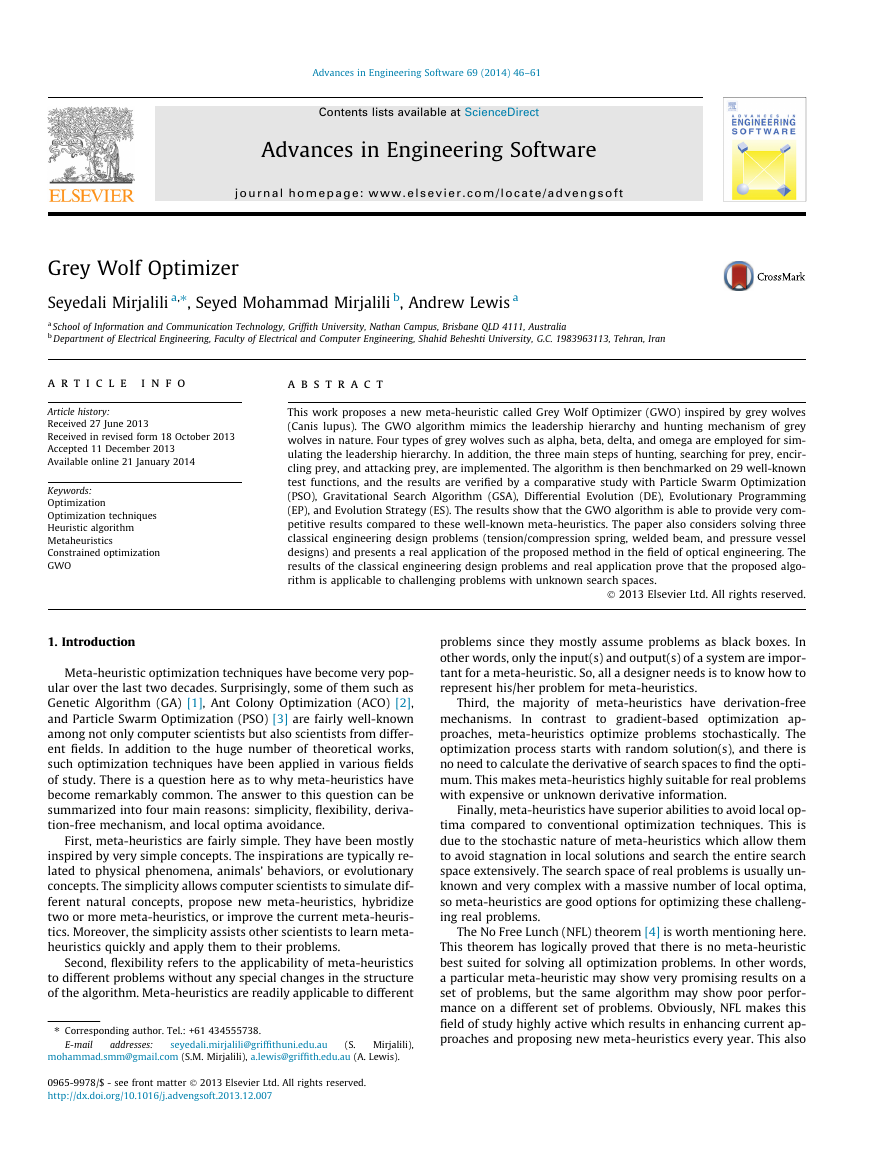Of particular interest is that they have a very strict social dominant hierarchy as shown in Fig. 1. The leaders are a male and a female, called alphas. The alpha is mostly responsible for making decisions about hunting, sleeping place, time to wake, and so on. The alpha’s decisions are dictated to the pack. However, some kind of democratic behavior has also been observed, in which an alpha follows the other wolves in the pack. In gatherings, the entire pack acknowledges the alpha by holding their tails down. The alpha wolf is also called the dominant wolf since his/her orders should be followed by the pack [46]. The alpha wolves are only allowed to mate in the pack. Interestingly, the alpha is not necessarily the strongest member of the pack but the best in terms of managing the pack. This shows that the organization and discipline of a pack is much more important than its strength. The second level in the hierarchy of grey wolves is beta. The be- tas are subordinate wolves that help the alpha in decision-making or other pack activities. The beta wolf can be either male or female, and he/she is probably the best candidate to be the alpha in case one of the alpha wolves passes away or becomes very old. The beta wolf should respect the alpha, but commands the other lower-level wolves as well. It plays the role of an advisor to the alpha and dis- cipliner for the pack. The beta reinforces the alpha’s commands throughout the pack and gives feedback to the alpha. The lowest ranking grey wolf is omega. The omega plays the role of scapegoat. Omega wolves always have to submit to all the other dominant wolves. They are the last wolves that are allowed to eat. It may seem the omega is not an important individual in the pack, but it has been observed that the whole pack face internal ﬁghting and problems in case of losing the omega. This is due to the venting of violence and frustration of all wolves by the ome- ga(s). This assists satisfying the entire pack and maintaining the dominance structure. In some cases the omega is also the babysit- ters in the pack. If a wolf is not an alpha, beta, or omega, he/she is called subor- dinate (or delta in some references). Delta wolves have to submit to alphas and betas, but they dominate the omega. Scouts, senti- nels, elders, hunters, and caretakers belong to this category. Scouts are responsible for watching the boundaries of the territory and warning the pack in case of any danger. Sentinels protect and guar- antee the safety of the pack. Elders are the experienced wolves who used to be alpha or beta. Hunters help the alphas and betas when hunting prey and providing food for the pack. Finally, the caretak- ers are responsible for caring for the weak, ill, and wounded wolves in the pack. 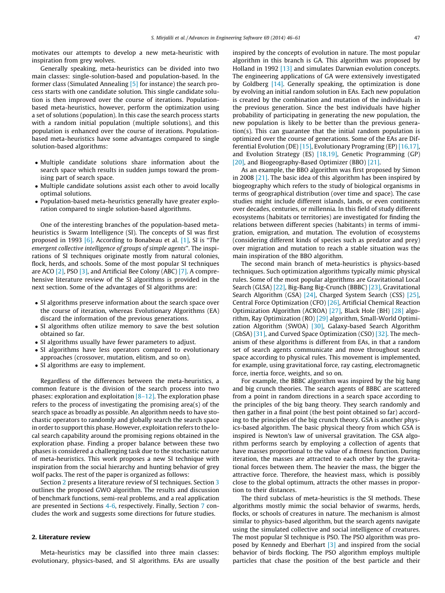In addition to the social hierarchy of wolves, group hunting is another interesting social behavior of grey wolves. According to Muro et al. [47] the main phases of grey wolf hunting are as follows: Tracking, chasing, and approaching the prey. Pursuing, encircling, and harassing the prey until it stops moving. Attack towards the prey. These steps are shown in Fig. 2. In this work this hunting technique and the social hierarchy of grey wolves are mathematically modeled in order to design GWO and perform optimization. Fig. 1. Hierarchy of grey wolf (dominance decreases from top down).

S. Mirjalili et al. / Advances in Engineering Software 69 (2014) 46–61 49 3.2. Mathematical model and algorithm In this subsection the mathematical models of the social hierar- chy, tracking, encircling, and attacking prey are provided. Then the GWO algorithm is outlined. 3.2.1. Social hierarchy In order to mathematically model the social hierarchy of wolves when designing GWO, we consider the ﬁttest solution as the alpha (a). Consequently, the second and third best solutions are named beta (b) and delta (d) respectively. The rest of the candidate solu- tions are assumed to be omega (x). In the GWO algorithm the hunting (optimization) is guided by a, b, and d. The x wolves fol- low these three wolves. 3.2.2. Encircling prey As mentioned above, grey wolves encircle prey during the hunt. In order to mathematically model encircling behavior the follow- ing equations are proposed: ~D ¼ j~C ~XpðtÞ ~XðtÞj ð3:1Þ ~Xðt þ 1Þ ¼ ~XpðtÞ ~A ~D ð3:2Þ where t indicates the current iteration, ~A and ~C are coefﬁcient vec- tors, ~Xp is the position vector of the prey, and ~X indicates the posi- tion vector of a grey wolf. The vectors ~A and ~C are calculated as follows: ~A ¼ 2~a ~r1 ~a ð3:3Þ ð3:4Þ ~C ¼ 2 ~r2 where components of ~a are linearly decreased from 2 to 0 over the course of iterations and r1, r2 are random vectors in [0,1]. 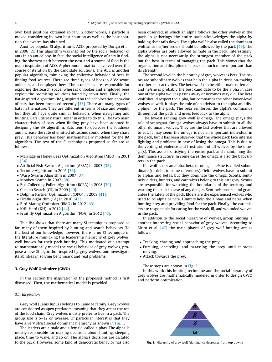To see the effects of Eqs. 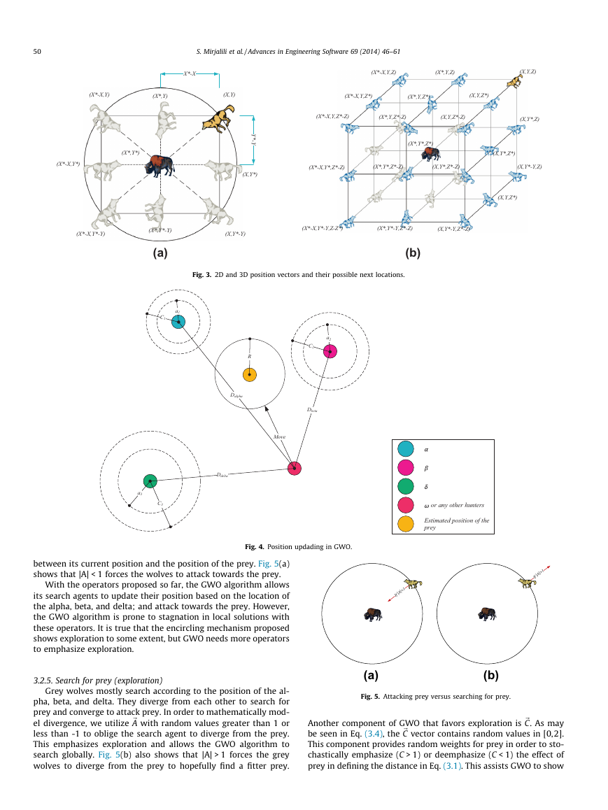(3.1) and (3.2), a two-dimensional po- sition vector and some of the possible neighbors are illustrated in Fig. 3(a). As can be seen in this ﬁgure, a grey wolf in the position of (X, Y) can update its position according to the position of the prey (X, Y). Different places around the best agent can be reached with respect to the current position by adjusting the value of ~A and ~C (X–X, Y) can be reached by setting vectors. For instance, ~A ¼ ð1; 0Þ and ~C ¼ ð1; 1Þ. The possible updated positions of a grey wolf in 3D space are depicted in Fig. 3(b). Note that the random vectors r1 and r2 allow wolves to reach any position between the points illustrated in Fig. 3. So a grey wolf can update its position in- side the space around the prey in any random location by using Eqs. (3.1) and (3.2). The same concept can be extended to a search space with n dimensions, and the grey wolves will move in hyper-cubes (or hy- per-spheres) around the best solution obtained so far. 3.2.3. Hunting Grey wolves have the ability to recognize the location of prey and encircle them. The hunt is usually guided by the alpha. The beta and delta might also participate in hunting occasionally. How- ever, in an abstract search space we have no idea about the loca- tion of the optimum (prey). In order to mathematically simulate the hunting behavior of grey wolves, we suppose that the alpha (best candidate solution) beta, and delta have better knowledge about the potential location of prey. Therefore, we save the ﬁrst three best solutions obtained so far and oblige the other search agents (including the omegas) to update their positions according to the position of the best search agents. The following formulas are proposed in this regard. 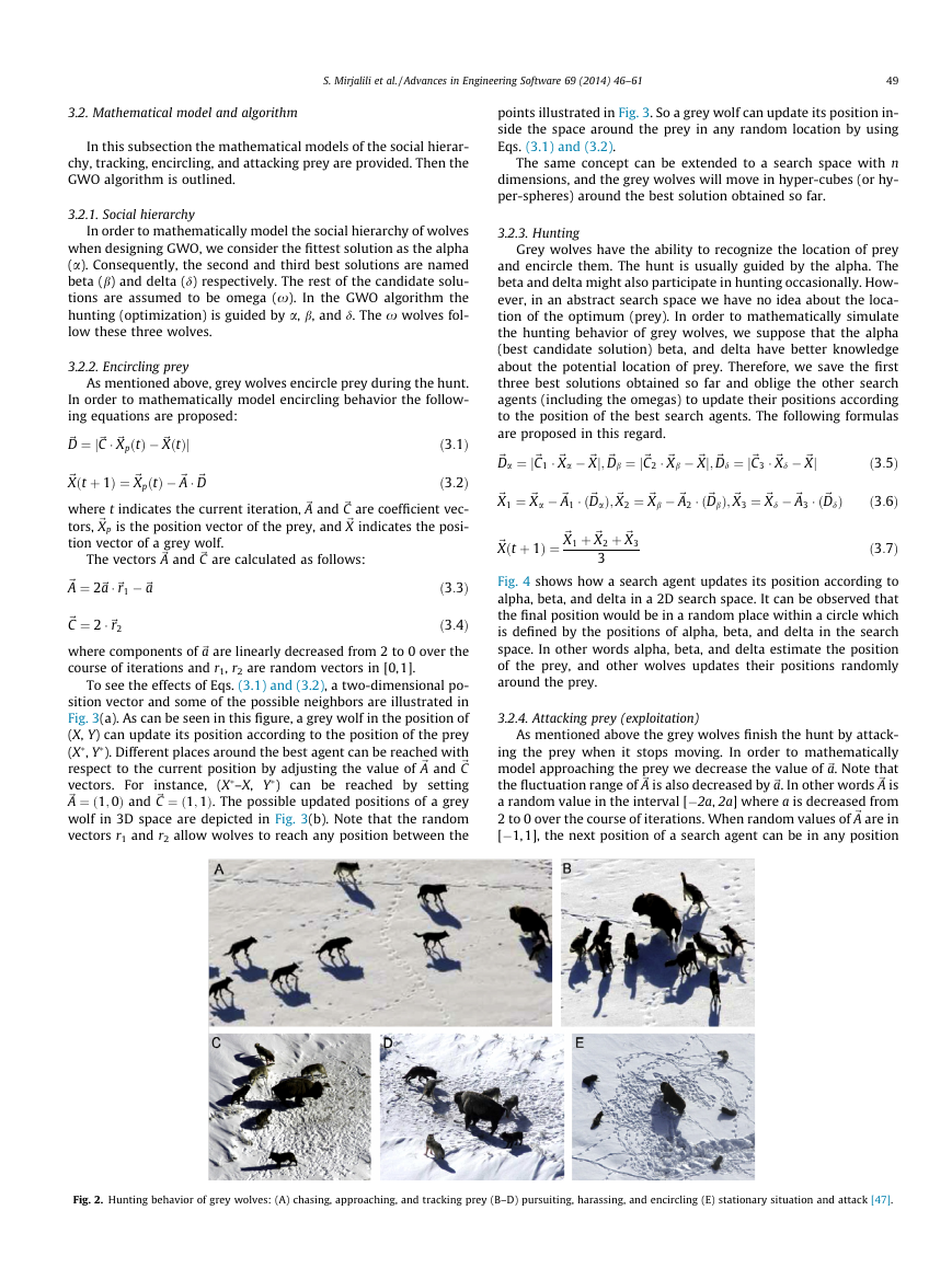~Da ¼ j~C1 ~Xa ~Xj; ~Db ¼ j~C2 ~Xb ~Xj; ~Dd ¼ j~C3 ~Xd ~Xj ð3:5Þ ~X1 ¼ ~Xa ~A1 ð~DaÞ; ~X2 ¼ ~Xb ~A2 ð~DbÞ; ~X3 ¼ ~Xd ~A3 ð~DdÞ ~Xðt þ 1Þ ¼ ~X1 þ ~X2 þ ~X3 3 ð3:6Þ ð3:7Þ Fig. 4 shows how a search agent updates its position according to alpha, beta, and delta in a 2D search space. It can be observed that the ﬁnal position would be in a random place within a circle which is deﬁned by the positions of alpha, beta, and delta in the search space. In other words alpha, beta, and delta estimate the position of the prey, and other wolves updates their positions randomly around the prey. 3.2.4. Attacking prey (exploitation) As mentioned above the grey wolves ﬁnish the hunt by attack- ing the prey when it stops moving. In order to mathematically model approaching the prey we decrease the value of ~a. Note that the ﬂuctuation range of ~A is also decreased by ~a. In other words ~A is a random value in the interval [2a, 2a] where a is decreased from 2 to 0 over the course of iterations. When random values of ~A are in [1,1], the next position of a search agent can be in any position Fig. 2. Hunting behavior of grey wolves: (A) chasing, approaching, and tracking prey (B–D) pursuiting, harassing, and encircling (E) stationary situation and attack [47].

50 S. Mirjalili et al. / Advances in Engineering Software 69 (2014) 46–61 X*-X (X*-X,Y,Z) (X*,Y,Z) (X,Y,Z) (X*-X,Y) (X*,Y) (X,Y) (X*-X,Y,Z*) (X*,Y,Z*) (X,Y,Z*) (X*-X,Y,Z*-Z) (X*,Y,Z*-Z) (X,Y,Z*-Z) (X,Y*,Z) (X*,Y*,Z*) (X,Y*,Z*) (X*-X,Y*,Z*-Z) (X*,Y*,Z*-Z) (X,Y*,Z*-Z) (X,Y*-Y,Z) Y * - Y (X,Y*) (X,Y,Z*) (X,Y*-Y) (X*-X,Y*-Y,Z-Z*) (X*,Y*-Y,Z*-Z) (X,Y*-Y,Z*-Z) (b) Fig. 3. 2D and 3D position vectors and their possible next locations. (X*,Y*) (X*-X,Y*) (X*-X,Y*-Y) (X*,Y*-Y) (a) a1 C1 R Dalpha a2 C2 Dbeta Move Ddelta a3 C3 Fig. 4. Position updading in GWO. between its current position and the position of the prey. Fig. 5(a) shows that |A| < 1 forces the wolves to attack towards the prey. With the operators proposed so far, the GWO algorithm allows its search agents to update their position based on the location of the alpha, beta, and delta; and attack towards the prey. However, the GWO algorithm is prone to stagnation in local solutions with these operators. It is true that the encircling mechanism proposed shows exploration to some extent, but GWO needs more operators to emphasize exploration. 3.2.5. Search for prey (exploration) Grey wolves mostly search according to the position of the al- pha, beta, and delta. They diverge from each other to search for prey and converge to attack prey. In order to mathematically mod- el divergence, we utilize ~A with random values greater than 1 or less than -1 to oblige the search agent to diverge from the prey. This emphasizes exploration and allows the GWO algorithm to search globally. Fig. 5(b) also shows that |A| > 1 forces the grey wolves to diverge from the prey to hopefully ﬁnd a ﬁtter prey. or any other hunters Estimated position of the prey If |A|< 1 If |A|> 1 (a) (b) Fig. 5. Attacking prey versus searching for prey. Another component of GWO that favors exploration is ~C. As may be seen in Eq. (3.4), the ~C vector contains random values in [0,2]. This component provides random weights for prey in order to sto- chastically emphasize (C > 1) or deemphasize (C < 1) the effect of prey in deﬁning the distance in Eq. (3.1). This assists GWO to show

S. Mirjalili et al. / Advances in Engineering Software 69 (2014) 46–61 51 a more random behavior throughout optimization, favoring explo- ration and local optima avoidance. It is worth mentioning here that C is not linearly decreased in contrast to A. We deliberately require C to provide random values at all times in order to emphasize exploration not only during initial iterations but also ﬁnal itera- tions. This component is very helpful in case of local optima stag- nation, especially in the ﬁnal iterations. The C vector can be also considered as the effect of obstacles to approaching prey in nature. Generally speaking, the obstacles in nature appear in the hunting paths of wolves and in fact prevent them from quickly and conveniently approaching prey. This is ex- actly what the vector C does. Depending on the position of a wolf, it can randomly give the prey a weight and make it harder and far- ther to reach for wolves, or vice versa. To sum up, the search process starts with creating a random population of grey wolves (candidate solutions) in the GWO algo- rithm. Over the course of iterations, alpha, beta, and delta wolves estimate the probable position of the prey. Each candidate solution updates its distance from the prey. The parameter a is decreased from 2 to 0 in order to emphasize exploration and exploitation, respectively. Candidate solutions tend to diverge from the prey when j~Aj > 1 and converge towards the prey when j~Aj < 1. Finally, the GWO algorithm is terminated by the satisfaction of an end criterion. 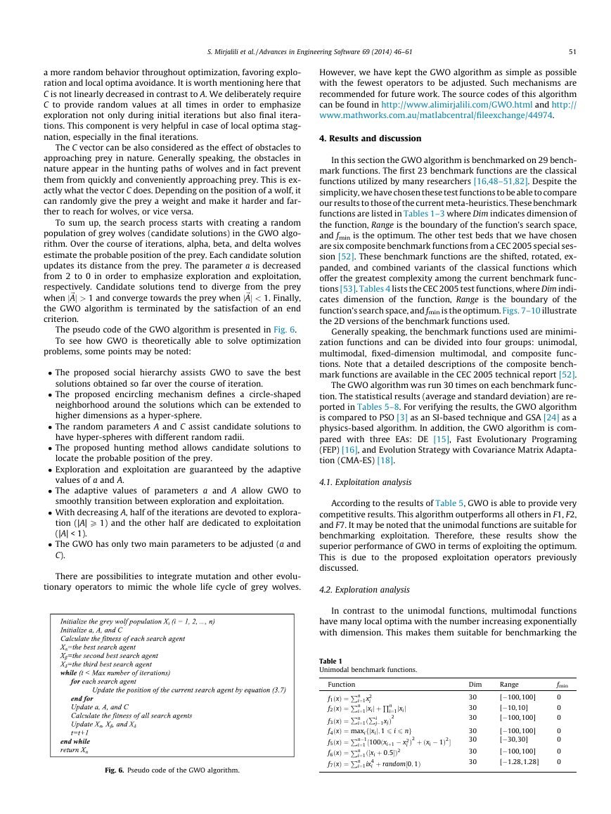The pseudo code of the GWO algorithm is presented in Fig. 6. To see how GWO is theoretically able to solve optimization problems, some points may be noted: The proposed social hierarchy assists GWO to save the best solutions obtained so far over the course of iteration. The proposed encircling mechanism deﬁnes a circle-shaped neighborhood around the solutions which can be extended to higher dimensions as a hyper-sphere. The random parameters A and C assist candidate solutions to have hyper-spheres with different random radii. The proposed hunting method allows candidate solutions to locate the probable position of the prey. Exploration and exploitation are guaranteed by the adaptive values of a and A. The adaptive values of parameters a and A allow GWO to smoothly transition between exploration and exploitation. With decreasing A, half of the iterations are devoted to explora- tion (|A| P 1) and the other half are dedicated to exploitation (|A| < 1). The GWO has only two main parameters to be adjusted (a and C). There are possibilities to integrate mutation and other evolu- tionary operators to mimic the whole life cycle of grey wolves. Fig. 6. Pseudo code of the GWO algorithm. However, we have kept the GWO algorithm as simple as possible with the fewest operators to be adjusted. Such mechanisms are recommended for future work. The source codes of this algorithm can be found in http://www.alimirjalili.com/GWO.html and http:// www.mathworks.com.au/matlabcentral/ﬁleexchange/44974. 4. Results and discussion In this section the GWO algorithm is benchmarked on 29 bench- mark functions. The ﬁrst 23 benchmark functions are the classical functions utilized by many researchers [16,48–51,82]. Despite the simplicity, we have chosen these test functions to be able to compare our results to those of the current meta-heuristics. These benchmark functions are listed in Tables 1–3 where Dim indicates dimension of the function, Range is the boundary of the function’s search space, and fmin is the optimum. The other test beds that we have chosen are six composite benchmark functions from a CEC 2005 special ses- sion [52]. These benchmark functions are the shifted, rotated, ex- panded, and combined variants of the classical functions which offer the greatest complexity among the current benchmark func- tions [53]. Tables 4 lists the CEC 2005 test functions, where Dim indi- cates dimension of the function, Range is the boundary of the function’s search space, and fmin is the optimum. Figs. 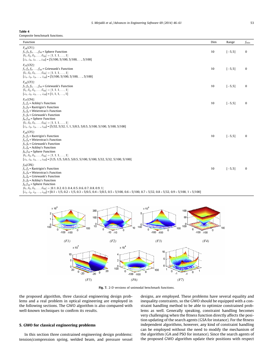7–10 illustrate the 2D versions of the benchmark functions used. Generally speaking, the benchmark functions used are minimi- zation functions and can be divided into four groups: unimodal, multimodal, ﬁxed-dimension multimodal, and composite func- tions. Note that a detailed descriptions of the composite bench- mark functions are available in the CEC 2005 technical report [52]. The GWO algorithm was run 30 times on each benchmark func- tion. The statistical results (average and standard deviation) are re- ported in Tables 5–8. For verifying the results, the GWO algorithm is compared to PSO [3] as an SI-based technique and GSA [24] as a physics-based algorithm. In addition, the GWO algorithm is com- pared with three EAs: DE [15], Fast Evolutionary Programing (FEP) [16], and Evolution Strategy with Covariance Matrix Adapta- tion (CMA-ES) [18]. 4.1. Exploitation analysis According to the results of Table 5, GWO is able to provide very competitive results. This algorithm outperforms all others in F1, F2, and F7. It may be noted that the unimodal functions are suitable for benchmarking exploitation. Therefore, these results show the superior performance of GWO in terms of exploiting the optimum. This is due to the proposed exploitation operators previously discussed. 4.2. Exploration analysis In contrast to the unimodal functions, multimodal functions have many local optima with the number increasing exponentially with dimension. This makes them suitable for benchmarking the Table 1 Unimodal benchmark functions. n Q i¼1jxij P Function P f1ðxÞ ¼ n i¼1x2 i P P i¼1jxij þ f2ðxÞ ¼ n i¼1ð f3ðxÞ ¼ j1xjÞ2 P f4ðxÞ ¼ maxifjxij; 1 6 i 6 ng P n1 f5ðxÞ ¼ i¼1 ½100ðxiþ1 x2 P f6ðxÞ ¼ i¼1ð½xi þ 0:5Þ2 n f7ðxÞ ¼ i¼1ix4 n n i i Þ2 þ ðxi 1Þ2 i þ random½0; 1Þ Dim 30 30 30 30 30 30 30 Range [100,100] [10,10] [100,100] [100,100] [30,30] [100,100] [1.28,1.28] fmin 0 0 0 0 0 0 0

52 S. Mirjalili et al. / Advances in Engineering Software 69 (2014) 46–61 Table 2 Multimodal benchmark functions. n n n n 4000 n i¼1x2 þ 20 þ e n f10 sinðpy1Þ þ exp 1 þ 1 P i¼1 cosð2pxiÞ ﬃﬃﬃﬃﬃﬃﬃ p P Function P Þ jxij i¼1 xi sinð F8ðxÞ ¼ q ﬃﬃﬃﬃﬃﬃﬃﬃﬃﬃﬃﬃﬃﬃﬃﬃﬃﬃﬃ P i 10 cosð2pxiÞ þ 10 i¼1½x2 F9ðxÞ ¼ Q P F10ðxÞ ¼ 20 exp 0:2 n 1 i¼1x2 ﬃ n i P F11ðxÞ ¼ 1 i n p i¼1 cos xi i n1 F12ðxÞ ¼ p i¼1 ðyi 1Þ2½1 þ 10 sin2ðpyiþ1Þ þ ðyn 1Þ2g þ yi ¼ 1 þ xiþ1 kðxi aÞm xi > a uðxi; a; k; mÞ ¼ a < xi < a 0 P kðxi aÞm xi < a P i¼1ðxi 1Þ2½1 þ sin2ð3pxi þ 1Þ þ ðxn 1Þ2½1 þ sin2ð2pxnÞg þ F13ðxÞ ¼ 0:1fsin2ð3px1Þ þ P P i h i¼1 sinðxiÞ sin i:x2 F14ðxÞ ¼ i p P P i¼1ðxi =bÞ2m 2e F15ðxÞ ¼ e n i¼1x2 i¼1 sin2ðxiÞ expð F16ðxÞ ¼ f½ Q ; m ¼ 10 P i¼1 cos2 xi; m ¼ 5 i Þg exp½ n i¼1x2 ﬃﬃﬃﬃﬃﬃﬃ jxij i¼1 sin2 8< : p 2m 4 n n n n i n n P i¼1uðxi; 10; 100; 4Þ n P i¼1uðxi; 5; 100; 4Þ n Dim 30 30 30 30 30 30 30 30 30 Range [500, 500] [5.12, 5.12] [32, 32] [600, 600] [50, 50] fmin 418.9829 5 0 0 0 0 [50, 50] [0,p] [20, 20] [10, 10] 0 4.687 1 1 Table 3 Fixed-dimension multimodal benchmark functions. 2 2 11 25 j¼1 P 1 P 1 i¼1ðxiaijÞ6 Function 500 þ F14ðxÞ ¼ 1 P jþ i þbix2Þ i¼1 ai x1ðb2 F15ðxÞ ¼ i þbix3þx4 b2 2 þ 4x4 1 þ x1x2 4x2 F16ðxÞ ¼ 4x2 1 þ 1 1 2:1x4 3 x6 2 þ 10 1 1 F17ðxÞ ¼ x2 5:1 1 þ 5 p x1 6 4p2 x2 8p P P F18ðxÞ ¼ ½1 þ ðx1 þ x2 þ 1Þ2ð19 14x1 þ 3x2 P P F19ðxÞ ¼ i¼1ci expð j¼1aijðxj pijÞ2Þ P i¼1ci expð F20ðxÞ ¼ j¼1aijðxj pijÞ2Þ P i¼1½ðX aiÞðX aiÞT þ ci1 F21ðxÞ ¼ P i¼1½ðX aiÞðX aiÞT þ ci1 F22ðxÞ ¼ i¼1½ðX aiÞðX aiÞT þ ci1 F23ðxÞ ¼ 10 2 4 3 4 6 5 7 cos x1 þ 10 1 14x2 þ 6x1x2 þ 3x2 2Þ ½30 þ ð2x1 3x2Þ2 ð18 32x1 þ 12x2 1 þ 48x2 36x1x2 þ 27x2 2Þ Dim Range 2 4 2 2 2 3 6 4 4 4 [65,65] [5,5] [5,5] [5,5] [2,2] [1, 3] [0, 1] [0, 10] [0, 10] [0, 10] fmin 1 0.00030 1.0316 0.398 3 3.86 3.32 10.1532 10.4028 10.5363 exploration ability of an algorithm. According to the results of Tables 6 and 7, GWO is able to provide very competitive results on the multimodal benchmark functions as well. This algorithm outperforms PSO and GSA on the majority of the multimodal func- tions. Moreover, GWO shows very competitive results compare to DE and FEP; and outperforms them occasionally. These results show that the GWO algorithm has merit in terms of exploration. 4.3. Local minima avoidance The fourth class of benchmark functions employed includes composite functions, generally very challenging test beds for meta-heuristic algorithms. So, exploration and exploitation can be simultaneously benchmarked by the composite functions. Moreover, the local optima avoidance of an algorithm can be examined due to the massive number of local optima in such test functions. According to Table 8, GWO outperforms all others on half of the composite benchmark functions. The GWO algorithm also provides very competitive results on the remaining composite benchmark functions. This demonstrates that GWO shows a good balance between exploration and exploitation that results in high local optima avoidance. This superior capability is due to the adap- tive value of A. As mentioned above, half of the iterations are de- voted to exploration (|A| P 1) and the rest to exploitation (|A| < 1). This mechanism assists GWO to provide very good explo- ration, local minima avoidance, and exploitation simultaneously. 4.4. Convergence behavior analysis In this subsection the convergence behavior of GWO is investi- gated. According to Berg et al. [54], there should be abrupt changes in the movement of search agents over the initial steps of optimi- zation. This assists a meta-heuristic to explore the search space extensively. Then, these changes should be reduced to emphasize exploitation at the end of optimization. In order to observe the con- vergence behavior of the GWO algorithm, the search history and trajectory of the ﬁrst search agent in its ﬁrst dimension are illus- trated in Fig. 11. The animated versions of this ﬁgure can be found in Supplementary Materials. Note that the benchmark functions are shifted in this section, and we used six search agents to ﬁnd the optima. The second column of Fig. 11 depicts the search history of the search agents. It may be observed that the search agents of GWO tend to extensively search promising regions of the search spaces and exploit the best one. In addition, the fourth column of Fig. 11 shows the trajectory of the ﬁrst particle, in which changes of the ﬁrst search agent in its ﬁrst dimension can be observed. It can be seen that there are abrupt changes in the initial steps of iterations which are decreased gradually over the course of iterations. According to Berg et al. [54], this behavior can guarantee that a SI algorithm eventually convergences to a point in search space. To sum up, the results verify the performance of the GWO algo- rithm in solving various benchmark functions compared to well- known meta-heuristics. To further investigate the performance of

S. Mirjalili et al. / Advances in Engineering Software 69 (2014) 46–61 53 Table 4 Composite benchmark functions. Function F24(CF1): f1, f2, f3, . . ., f10 = Sphere Function ½,1; ,2; ,3; . . . ; ,10 ¼ ½1; 1; 1; . . . ; 1 [k1, k2, k3 . . ., k10] = [5/100, 5/100, 5/100, . . ., 5/100] F25(CF2): f1, f2, f3, . . ., f10 = Griewank’s Function ½,1; ,2; ,3; . . . ; ,10 ¼ ½1; 1; 1; . . . ; 1 [k1, k2, k3, . . ., k10] = [5/100, 5/100, 5/100, . . ., 5/100] F26(CF3): f1, f2, f3, . . ., f10 = Griewank’s Function ½,1; ,2; ,3; . . . ; ,10 ¼ ½1; 1; 1; . . . ; 1 [k1, k2, k3, . . ., k10] = [1, 1, 1, . . ., 1] F27(CF4): f1, f2 = Ackley’s Function f3, f4 = Rastrigin’s Function f5, f6 = Weierstras’s Function f7, f8 = Griewank’s Function f9, f10 = Sphere Function ½,1; ,2; ,3; . . . ; ,10 ¼ ½1; 1; 1; . . . ; 1 [k1, k2, k3, . . ., k10] = [5/32, 5/32, 1, 1, 5/0.5, 5/0.5, 5/100, 5/100, 5/100, 5/100] F28(CF5): f1, f2 = Rastrigin’s Function f3, f4 = Weierstras’s Function f5, f6 = Griewank’s Function f7, f8 = Ackley’s Function f9, f10 = Sphere Function ½,1; ,2; ,3; . . . ; ,10 ¼ ½1; 1; 1; . . . ; 1 [k1, k2, k3, . . ., k10] = [1/5, 1/5, 5/0.5, 5/0.5, 5/100, 5/100, 5/32, 5/32, 5/100, 5/100] f29(CF6): f1, f2 = Rastrigin’s Function f3, f4 = Weierstras’s Function f5, f6 = Griewank’s Function f7, f8 = Ackley’s Function f9, f10 = Sphere Function ½,1; ,2; ,3; . . . ; ,10 ¼ ½0:1; 0:2; 0:3; 0:4; 0:5; 0:6; 0:7; 0:8; 0:9; 1 [k1, k2, k3, . . ., k10] = [0.1 1/5, 0.2 1/5, 0.3 5/0.5, 0.4 5/0.5, 0.5 5/100, 0.6 5/100, 0.7 5/32, 0.8 5/32, 0.9 5/100, 1 5/100] Dim Range fmin 10 10 10 10 [5, 5] [5, 5] [5, 5] [5, 5] 10 [5, 5] 10 [5, 5] 0 0 0 0 0 0 (F1) (F2) (F3) (F4) (F5) (F6) (F7) Fig. 7. 2-D versions of unimodal benchmark functions. the proposed algorithm, three classical engineering design prob- lems and a real problem in optical engineering are employed in the following sections. The GWO algorithm is also compared with well-known techniques to conﬁrm its results. 5. GWO for classical engineering problems In this section three constrained engineering design problems: tension/compression spring, welded beam, and pressure vessel designs, are employed. These problems have several equality and inequality constraints, so the GWO should be equipped with a con- straint handling method to be able to optimize constrained prob- lems as well. Generally speaking, constraint handling becomes very challenging when the ﬁtness function directly affects the posi- tion updating of the search agents (GSA for instance). For the ﬁtness independent algorithms, however, any kind of constraint handling can be employed without the need to modify the mechanism of the algorithm (GA and PSO for instance). Since the search agents of the proposed GWO algorithm update their positions with respect

分享到：

赞收藏

资料库

Grey Wolf Optimizer（狼群算法最早的一篇文章）GWO.pdf

相关推荐

行业

热门标签

最新资料