5
1
0
2
t
c
O
7
1
]
G
L
.
s
c
[
4
v
9
1
0
0
0
.
6
0
5
1
:
v
i
X
r
a
A Critical Review of Recurrent Neural Networks
for Sequence Learning
Zachary C. Lipton
John Berkowitz
zlipton@cs.ucsd.edu
jaberkow@physics.ucsd.edu
Charles Elkan
elkan@cs.ucsd.edu
June 5th, 2015
Abstract
Countless learning tasks require dealing with sequential data. Image
captioning, speech synthesis, and music generation all require that a model
produce outputs that are sequences. In other domains, such as time series
prediction, video analysis, and musical information retrieval, a model must
learn from inputs that are sequences. Interactive tasks, such as translat-
ing natural language, engaging in dialogue, and controlling a robot, often
demand both capabilities. Recurrent neural networks (RNNs) are connec-
tionist models that capture the dynamics of sequences via cycles in the
network of nodes. Unlike standard feedforward neural networks, recurrent
networks retain a state that can represent information from an arbitrarily
long context window. Although recurrent neural networks have tradition-
ally been difficult to train, and often contain millions of parameters, recent
advances in network architectures, optimization techniques, and paral-
lel computation have enabled successful large-scale learning with them.
In recent years, systems based on long short-term memory (LSTM) and
bidirectional (BRNN) architectures have demonstrated ground-breaking
performance on tasks as varied as image captioning, language translation,
and handwriting recognition.
In this survey, we review and synthesize
the research that over the past three decades first yielded and then made
practical these powerful learning models. When appropriate, we reconcile
conflicting notation and nomenclature. Our goal is to provide a self-
contained explication of the state of the art together with a historical
perspective and references to primary research.
1
Introduction
Neural networks are powerful learning models that achieve state-of-the-art re-
sults in a wide range of supervised and unsupervised machine learning tasks.
1
�
They are suited especially well for machine perception tasks, where the raw un-
derlying features are not individually interpretable. This success is attributed
to their ability to learn hierarchical representations, unlike traditional meth-
ods that rely upon hand-engineered features [Farabet et al., 2013]. Over the
past several years, storage has become more affordable, datasets have grown
far larger, and the field of parallel computing has advanced considerably.
In
the setting of large datasets, simple linear models tend to under-fit, and often
under-utilize computing resources. Deep learning methods, in particular those
based on deep belief networks (DNNs), which are greedily built by stacking re-
stricted Boltzmann machines, and convolutional neural networks, which exploit
the local dependency of visual information, have demonstrated record-setting
results on many important applications.
However, despite their power, standard neural networks have limitations.
Most notably, they rely on the assumption of independence among the training
and test examples. After each example (data point) is processed, the entire state
of the network is lost. If each example is generated independently, this presents
no problem. But if data points are related in time or space, this is unaccept-
able. Frames from video, snippets of audio, and words pulled from sentences,
represent settings where the independence assumption fails. Additionally, stan-
dard networks generally rely on examples being vectors of fixed length. Thus
it is desirable to extend these powerful learning tools to model data with tem-
poral or sequential structure and varying length inputs and outputs, especially
in the many domains where neural networks are already the state of the art.
Recurrent neural networks (RNNs) are connectionist models with the ability to
selectively pass information across sequence steps, while processing sequential
data one element at a time. Thus they can model input and/or output con-
sisting of sequences of elements that are not independent. Further, recurrent
neural networks can simultaneously model sequential and time dependencies on
multiple scales.
In the following subsections, we explain the fundamental reasons why recur-
rent neural networks are worth investigating. To be clear, we are motivated by
a desire to achieve empirical results. This motivation warrants clarification be-
cause recurrent networks have roots in both cognitive modeling and supervised
machine learning. Owing to this difference of perspectives, many published pa-
pers have different aims and priorities. In many foundational papers, generally
published in cognitive science and computational neuroscience journals, such as
[Hopfield, 1982, Jordan, 1986, Elman, 1990], biologically plausible mechanisms
are emphasized.
In other papers [Schuster and Paliwal, 1997, Socher et al.,
2014, Karpathy and Fei-Fei, 2014], biological inspiration is downplayed in favor
of achieving empirical results on important tasks and datasets. This review
is motivated by practical results rather than biological plausibility, but where
appropriate, we draw connections to relevant concepts in neuroscience. Given
the empirical aim, we now address three significant questions that one might
reasonably want answered before reading further.
2
�
1.1 Why model sequentiality explicitly?
In light of the practical success and economic value of sequence-agnostic models,
this is a fair question. Support vector machines, logistic regression, and feedfor-
ward networks have proved immensely useful without explicitly modeling time.
Arguably, it is precisely the assumption of independence that has led to much
recent progress in machine learning. Further, many models implicitly capture
time by concatenating each input with some number of its immediate prede-
cessors and successors, presenting the machine learning model with a sliding
window of context about each point of interest. This approach has been used
with deep belief nets for speech modeling by Maas et al. [2012].
Unfortunately, despite the usefulness of the independence assumption, it
precludes modeling long-range dependencies. For example, a model trained
using a finite-length context window of length 5 could never be trained to answer
the simple question, “what was the data point seen six time steps ago?” For
a practical application such as call center automation, such a limited system
might learn to route calls, but could never participate with complete success
in an extended dialogue. Since the earliest conception of artificial intelligence,
researchers have sought to build systems that interact with humans in time. In
Alan Turing’s groundbreaking paper Computing Machinery and Intelligence, he
proposes an “imitation game” which judges a machine’s intelligence by its ability
to convincingly engage in dialogue [Turing, 1950]. Besides dialogue systems,
modern interactive systems of economic importance include self-driving cars
and robotic surgery, among others. Without an explicit model of sequentiality
or time, it seems unlikely that any combination of classifiers or regressors can
be cobbled together to provide this functionality.
1.2 Why not use Markov models?
Recurrent neural networks are not the only models capable of representing time
dependencies. Markov chains, which model transitions between states in an
observed sequence, were first described by the mathematician Andrey Markov
in 1906. Hidden Markov models (HMMs), which model an observed sequence
as probabilistically dependent upon a sequence of unobserved states, were de-
scribed in the 1950s and have been widely studied since the 1960s [Stratonovich,
1960]. However, traditional Markov model approaches are limited because their
states must be drawn from a modestly sized discrete state space S. The dynamic
programming algorithm that is used to perform efficient inference with hidden
Markov models scales in time O(|S|2) [Viterbi, 1967]. Further, the transition
table capturing the probability of moving between any two time-adjacent states
is of size |S|2. Thus, standard operations become infeasible with an HMM when
the set of possible hidden states grows large. Further, each hidden state can
depend only on the immediately previous state. While it is possible to extend a
Markov model to account for a larger context window by creating a new state
space equal to the cross product of the possible states at each time in the win-
dow, this procedure grows the state space exponentially with the size of the
3
�
window, rendering Markov models computationally impractical for modeling
long-range dependencies [Graves et al., 2014].
Given the limitations of Markov models, we ought to explain why it is rea-
sonable that connectionist models, i.e., artificial neural networks, should fare
better. First, recurrent neural networks can capture long-range time depen-
dencies, overcoming the chief limitation of Markov models. This point requires
a careful explanation. As in Markov models, any state in a traditional RNN
depends only on the current input as well as on the state of the network at the
previous time step.1 However, the hidden state at any time step can contain
information from a nearly arbitrarily long context window. This is possible be-
cause the number of distinct states that can be represented in a hidden layer of
nodes grows exponentially with the number of nodes in the layer. Even if each
node took only binary values, the network could represent 2N states where N is
the number of nodes in the hidden layer. When the value of each node is a real
number, a network can represent even more distinct states. While the potential
expressive power of a network grows exponentially with the number of nodes,
the complexity of both inference and training grows at most quadratically.
1.3 Are RNNs too expressive?
Finite-sized RNNs with nonlinear activations are a rich family of models, capa-
ble of nearly arbitrary computation. A well-known result is that a finite-sized
recurrent neural network with sigmoidal activation functions can simulate a uni-
versal Turing machine [Siegelmann and Sontag, 1991]. The capability of RNNs
to perform arbitrary computation demonstrates their expressive power, but one
could argue that the C programming language is equally capable of expressing
arbitrary programs. And yet there are no papers claiming that the invention of
C represents a panacea for machine learning. A fundamental reason is there is
no simple way of efficiently exploring the space of C programs. In particular,
there is no general way to calculate the gradient of an arbitrary C program to
minimize a chosen loss function. Moreover, given any finite dataset, there exist
countless programs which overfit the dataset, generating desired training output
but failing to generalize to test examples.
Why then should RNNs suffer less from similar problems? First, given any
fixed architecture (set of nodes, edges, and activation functions), the recurrent
neural networks with this architecture are differentiable end to end. The deriva-
tive of the loss function can be calculated with respect to each of the parameters
(weights) in the model. Thus, RNNs are amenable to gradient-based training.
Second, while the Turing-completeness of RNNs is an impressive property, given
a fixed-size RNN with a specific architecture, it is not actually possible to re-
produce any arbitrary program. Further, unlike a program composed in C, a
recurrent neural network can be regularized via standard techniques that help
1 While traditional RNNs only model the dependence of the current state on the previous
state, bidirectional recurrent neural networks (BRNNs) [Schuster and Paliwal, 1997] extend
RNNs to model dependence on both past states and future states.
4
�
prevent overfitting, such as weight decay, dropout, and limiting the degrees of
freedom.
1.4 Comparison to prior literature
The literature on recurrent neural networks can seem impenetrable to the unini-
tiated. Shorter papers assume familiarity with a large body of background lit-
erature, while diagrams are frequently underspecified, failing to indicate which
edges span time steps and which do not. Jargon abounds, and notation is in-
consistent across papers or overloaded within one paper. Readers are frequently
in the unenviable position of having to synthesize conflicting information across
many papers in order to understand just one. For example, in many papers sub-
scripts index both nodes and time steps. In others, h simultaneously stands for a
link function and a layer of hidden nodes. The variable t simultaneously stands
for both time indices and targets, sometimes in the same equation. Many excel-
lent research papers have appeared recently, but clear reviews of the recurrent
neural network literature are rare.
Among the most useful resources are a recent book on supervised sequence
labeling with recurrent neural networks [Graves, 2012] and an earlier doctoral
thesis [Gers, 2001]. A recent survey covers recurrent neural nets for language
modeling [De Mulder et al., 2015]. Various authors focus on specific technical
aspects; for example Pearlmutter [1995] surveys gradient calculations in contin-
uous time recurrent neural networks. In the present review paper, we aim to
provide a readable, intuitive, consistently notated, and reasonably comprehen-
sive but selective survey of research on recurrent neural networks for learning
with sequences. We emphasize architectures, algorithms, and results, but we
aim also to distill the intuitions that have guided this largely heuristic and
empirical field. In addition to concrete modeling details, we offer qualitative ar-
guments, a historical perspective, and comparisons to alternative methodologies
where appropriate.
2 Background
This section introduces formal notation and provides a brief background on
neural networks in general.
2.1 Sequences
The input to an RNN is a sequence, and/or its target is a sequence. An input
sequence can be denoted (x(1), x(2), ..., x(T )) where each data point x(t) is a real-
valued vector. Similarly, a target sequence can be denoted (y(1), y(2), ..., y(T )).
A training set typically is a set of examples where each example is an (input
sequence, target sequence) pair, although commonly either the input or the
output may be a single data point. Sequences may be of finite or countably
infinite length. When they are finite, the maximum time index of the sequence
5
�
is called T . RNNs are not limited to time-based sequences. They have been
used successfully on non-temporal sequence data, including genetic data [Baldi
and Pollastri, 2003]. However, in many important applications of RNNs, the
sequences have an explicit or implicit temporal aspect. While we often refer to
time in this survey, the methods described here are applicable to non-temporal
as well as to temporal tasks.
Using temporal terminology, an input sequence consists of data points x(t)
that arrive in a discrete sequence of time steps indexed by t. A target sequence
consists of data points y(t). We use superscripts with parentheses for time, and
not subscripts, to prevent confusion between sequence steps and indices of nodes
in a network. When a model produces predicted data points, these are labeled
ˆy(t).
The time-indexed data points may be equally spaced samples from a con-
tinuous real-world process. Examples include the still images that comprise
the frames of videos or the discrete amplitudes sampled at fixed intervals that
comprise audio recordings. The time steps may also be ordinal, with no exact
correspondence to durations. In fact, RNNs are frequently applied to domains
where sequences have a defined order but no explicit notion of time. This is
the case with natural language. In the word sequence “John Coltrane plays the
saxophone”, x(1) = John, x(2) = Coltrane, etc.
2.2 Neural networks
Neural networks are biologically inspired models of computation. Generally,
a neural network consists of a set of artificial neurons, commonly referred to
as nodes or units, and a set of directed edges between them, which intuitively
represent the synapses in a biological neural network. Associated with each
neuron j is an activation function lj(·), which is sometimes called a link function.
We use the notation lj and not hj, unlike some other papers, to distinguish the
activation function from the values of the hidden nodes in a network, which, as
a vector, is commonly notated h in the literature.
Associated with each edge from node j to j is a weight wjj. Following
the convention adopted in several foundational papers [Hochreiter and Schmid-
huber, 1997, Gers et al., 2000, Gers, 2001, Sutskever et al., 2011], we index
neurons with j and j, and wjj denotes the “to-from” weight corresponding to
the directed edge to node j from node j. It is important to note that in many
references the indices are flipped and wjj = wjj denotes the “from-to” weight
on the directed edge from the node j to the node j, as in lecture notes by Elkan
[2015] and in Wikipedia [2015].
The value vj of each neuron j is calculated by applying its activation function
to a weighted sum of the values of its input nodes (Figure 1):
j
.
vj = lj
wjj · vj
For convenience, we term the weighted sum inside the parentheses the incoming
6
�
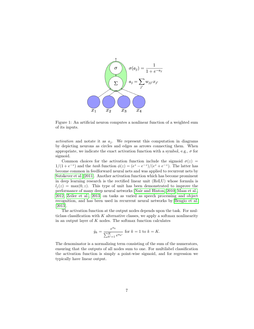
Figure 1: An artificial neuron computes a nonlinear function of a weighted sum
of its inputs.
activation and notate it as aj. We represent this computation in diagrams
by depicting neurons as circles and edges as arrows connecting them. When
appropriate, we indicate the exact activation function with a symbol, e.g., σ for
sigmoid.
Common choices for the activation function include the sigmoid σ(z) =
1/(1 + e−z) and the tanh function φ(z) = (ez − e−z)/(ez + e−z). The latter has
become common in feedforward neural nets and was applied to recurrent nets by
Sutskever et al. [2011]. Another activation function which has become prominent
in deep learning research is the rectified linear unit (ReLU) whose formula is
lj(z) = max(0, z). This type of unit has been demonstrated to improve the
performance of many deep neural networks [Nair and Hinton, 2010, Maas et al.,
2012, Zeiler et al., 2013] on tasks as varied as speech processing and object
recognition, and has been used in recurrent neural networks by Bengio et al.
[2013].
The activation function at the output nodes depends upon the task. For mul-
ticlass classification with K alternative classes, we apply a softmax nonlinearity
in an output layer of K nodes. The softmax function calculates
eakK
k=1 eak
ˆyk =
for k = 1 to k = K.
The denominator is a normalizing term consisting of the sum of the numerators,
ensuring that the outputs of all nodes sum to one. For multilabel classification
the activation function is simply a point-wise sigmoid, and for regression we
typically have linear output.
7
�
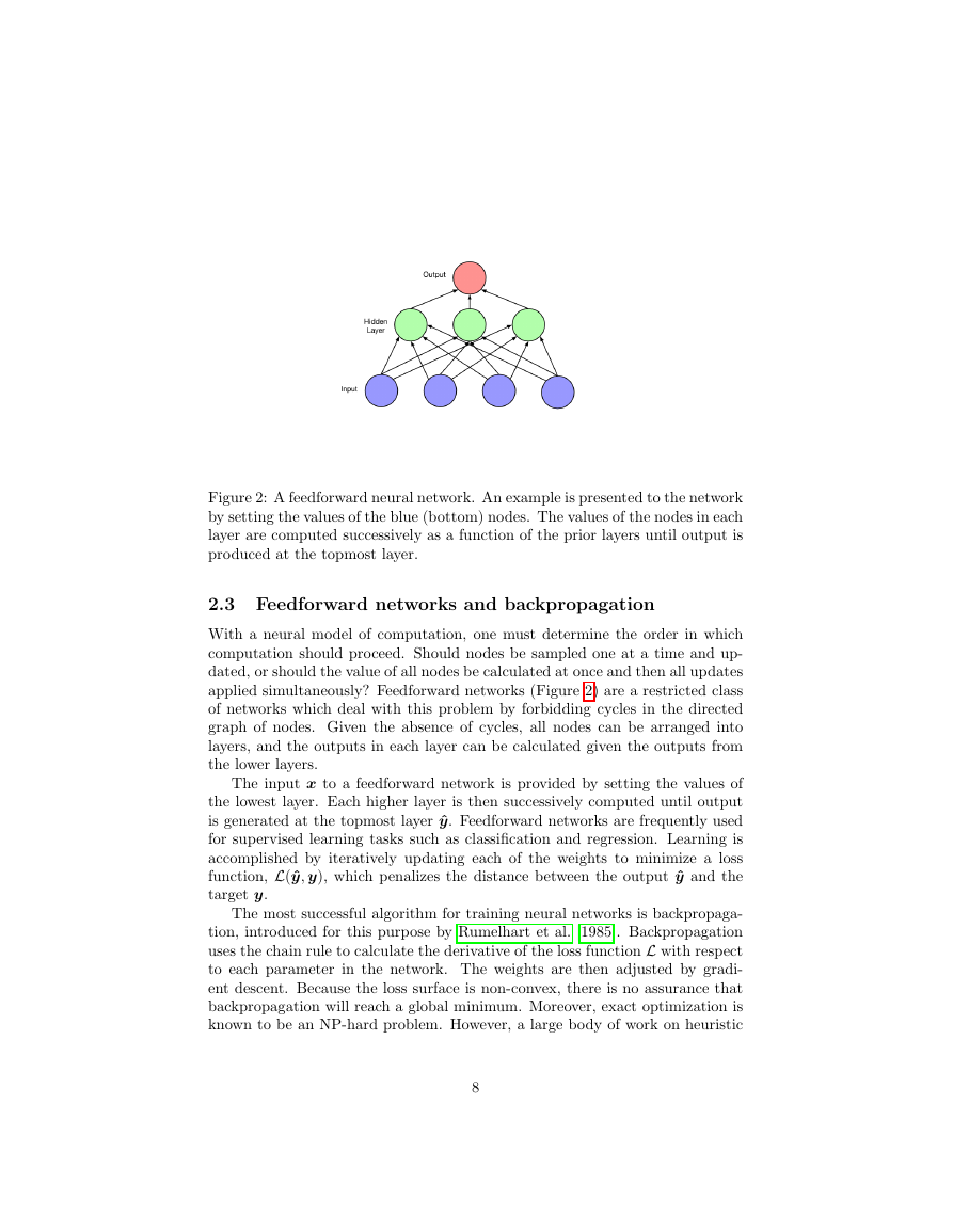
Figure 2: A feedforward neural network. An example is presented to the network
by setting the values of the blue (bottom) nodes. The values of the nodes in each
layer are computed successively as a function of the prior layers until output is
produced at the topmost layer.
2.3 Feedforward networks and backpropagation
With a neural model of computation, one must determine the order in which
computation should proceed. Should nodes be sampled one at a time and up-
dated, or should the value of all nodes be calculated at once and then all updates
applied simultaneously? Feedforward networks (Figure 2) are a restricted class
of networks which deal with this problem by forbidding cycles in the directed
graph of nodes. Given the absence of cycles, all nodes can be arranged into
layers, and the outputs in each layer can be calculated given the outputs from
the lower layers.
The input x to a feedforward network is provided by setting the values of
the lowest layer. Each higher layer is then successively computed until output
is generated at the topmost layer ˆy. Feedforward networks are frequently used
for supervised learning tasks such as classification and regression. Learning is
accomplished by iteratively updating each of the weights to minimize a loss
function, L(ˆy, y), which penalizes the distance between the output ˆy and the
target y.
The most successful algorithm for training neural networks is backpropaga-
tion, introduced for this purpose by Rumelhart et al. [1985]. Backpropagation
uses the chain rule to calculate the derivative of the loss function L with respect
to each parameter in the network. The weights are then adjusted by gradi-
ent descent. Because the loss surface is non-convex, there is no assurance that
backpropagation will reach a global minimum. Moreover, exact optimization is
known to be an NP-hard problem. However, a large body of work on heuristic
8
�


 2023年江西萍乡中考道德与法治真题及答案.doc
 2012年重庆南川中考生物真题及答案.doc
 2013年江西师范大学地理学综合及文艺理论基础考研真题.doc
 2020年四川甘孜小升初语文真题及答案I卷.doc
 2020年注册岩土工程师专业基础考试真题及答案.doc
 2023-2024学年福建省厦门市九年级上学期数学月考试题及答案.doc
 2021-2022学年辽宁省沈阳市大东区九年级上学期语文期末试题及答案.doc
 2022-2023学年北京东城区初三第一学期物理期末试卷及答案.doc
 2018上半年江西教师资格初中地理学科知识与教学能力真题及答案.doc
 2012年河北国家公务员申论考试真题及答案-省级.doc
 2020-2021学年江苏省扬州市江都区邵樊片九年级上学期数学第一次质量检测试题及答案.doc
 2022下半年黑龙江教师资格证中学综合素质真题及答案.doc