MOTION BLUR KERNEL ESTIMATION VIA SALIENT EDGES AND LOW RANK PRIOR
Jinshan Pan†, Risheng Liu‡§, Zhixun Su†, and Guili Liu†
† School of Mathematical Sciences, Dalian University of Technology, China
‡ School of Software Technology, Dalian University of Technology, China
Basic Teaching and Research Department, Harbin Finance University, China
State Key Laboratory of Novel Software Technology, Nanjing University, China
§ Faculty of Electronic Information and Electrical Engineering, Dalian University of Technology, China
ABSTRACT
Blind image deblurring, i.e., estimating a blur kernel from a
single input blurred image is a severely ill-posed problem. In
this paper, we show how to effectively apply low rank prior
to blind image deblurring and then propose a new algorithm
which combines salient edges and low rank prior. Salient
edges provide reliable edge information for kernel estimation,
while low rank prior provides data-authentic priors for the la-
tent image. When estimating the kernel, the salient edges are
extracted from an intermediate latent image solved by com-
bining the predicted edges and low rank prior, which help pre-
serve more useful edges than previous deconvolution methods
do. By solving the blind image deblurring problem in this
fashion, high-quality blur kernels can be obtained. Extensive
experiments testify to the superiority of the proposed method
over state-of-the-art algorithms, both qualitatively and quan-
titatively.
Index Terms— Blind image deblurring, low rank prior,
salient edges, kernel estimation, image restoration
1. INTRODUCTION
Blind image deblurring has gained considerable attention and
achieved great success in recent years. The formation process
of image blur is usually modeled as:
B = I ∗ k + ε,
(1)
where B, I, k and ε represent the blurred image, latent image,
blur kernel, and the additive noise, respectively. ∗ denotes
the convolution operator. It is a well-known ill-posed inverse
problem, which requires regularization in order to obtain a
high quality latent image.
1.1. Related Work
In order to make blind deblurring more tractable, early ap-
proaches imposed constraints on motion blur kernels [1, 2],
This work is partially supported by the NSFC (Nos. 61300086,
61173103, and 91230103), National Science and Technology Major
Project (No. 2013ZX04005021), China Postdoctoral Science Foundation
(No. 2013M530917), the Fundamental Research Funds for the Central Uni-
versities (No. DUT12RC(3)67), and the Open Project Program of the State
Key Laboratory of CAD&CG, Zhejiang University (No. A1404).
and the solutions can be usually obtained by maximum a pos-
terior (MAP) approach.
Recently, Fergus et al. [3] proposed a zero-mean Mix-
ture of Gaussian to fit the distribution of natural image gra-
dients. Levin et al. [4, 5] proposed a hyper-Laplacian prior to
fit the distribution of natural image gradients. However, be-
cause naive MAP inference could fail on natural images, they
maximized marginalized distributions to get a better solution.
Another group of methods still followed the line of alter-
ing the naive MAP framework to estimate the blur kernels.
To avoid and overcome the naive limitations of MAP, a va-
riety of strategies have been proposed. Shan et al. [6] used a
certain parametric model to approximate the heavy-tailed nat-
ural image prior. Moreover, to avoid the delta kernel solution,
they used a large regularization weight to suppress insignifi-
cant structures and preserve strong ones. Krishnan et al. [7]
proposed a normalized sparsity prior, i.e., 1/2 regularizer.
This new regularizer favors latent images over blurred ones.
Joshi et al. [8] and Cho et al. [9] directly restored sharp edges
from blurred images and relied on them to estimate blur ker-
nels. The works [10, 11, 12] employed shock filter to predict
the sharp edges for kernel estimation. Cho and Lee [10] per-
formed bilateral filter and edge thresholding at each iteration
to preserve the sharp edges. The kernel estimation process
was achieved by a coarse-to-fine strategy. Xu and Jia [11]
extended the sharp edges selection method [10] and selected
the large scale edges for kernel estimation. Pan et al. [12]
went a further step. They proposed an adaptive edge selection
method and an effective gradient constraint for kernel estima-
tion. Sun et al. [13] employed patch priors to restore useful
edges for kernel estimation. These schemes have been exten-
sively validated in blind image deblurring. To avoid ad-hoc
edge selection step, Xu et al. [14] and Pan and Su [15] pro-
posed 0-regularized kernel estimation. Due to the properties
of 0-norm, these methods are able to select large scale edges
for kernel estimation.
Sparse representation as a new powerful image prior has
also been employed in blind deblurring [16, 17, 18]. Because
sparse representation is able to provide data-authentic priors
�
in the kernel estimation, these methods have also achieved
state-of-the-art results.
1.2. Our Contribution
In this paper, we find that although the sharp edges are able to
help kernel estimation, if the priors imposed on the interme-
diate latent images are improper, the accuracy of kernel esti-
mates are still affected by the salient edges extracted from in-
termediate latent images. Based on above analysis, we in this
paper propose a robust motion blur kernel estimation method
via salient edges and low rank prior. Salient edges are able to
avoid the delta kernels, while the low rank prior used in the
intermediate latent image restoration can provide more useful
data for the kernel estimation. Although low rank prior has
been successfully applied to many computer vision problems,
to the best of our knowledge, few algorithms utilize low rank
prior for kernel estimation.
2. KERNEL ESTIMATION VIA SALIENT EDGES
AND LOW RANK PRIOR
The proposed kernel estimation is based on the improved
MAP framework. It is achieved by iteratively solving latent
image restoration (Section 2.1) and kernel estimation (Sec-
tion 2.2).
2.1. Intermediate Latent Image Restoration via Low
Rank Prior
Intermediate latent image restoration plays a critical role in
kernel estimation process, because it provides data when es-
timating blur kernels. In this section, we will propose a new
robust intermediate latent image estimation method.
Sparse representation and nonlocal self-similarity have
In
been successfully used for image restoration problems.
these methods,
images are often decomposed into small
patches to better fit the sparse representation assumption [19]
or generate the weights by nonlocal neighboring patches [20].
The works [21, 22] provided the connection among the sparse
representation, nonlocal self-similarity, and low rank approx-
imation. Moreover, Dong et al. [21] proposed the following
model to remove the noise in the image:
min
X
F + λX∗,
Y − X2
(2)
where Y = [y1, y2, . . . , yN ] ∈ R
n×N is a set of similar im-
age patches with noise, X denotes the restored image patches
without noise, and X∗ denotes the nuclear norm of X, i.e.,
the sum of the singular values of the matrix X. Model (2) is
very effective in image denoising [21].
Inspired by the work [21], we employ the low rank prior to
guide the intermediate latent image restoration. Our restora-
tion model is defined as
I ∗ k − B2
2 + β∇I − ∇S2
min
I,L
(3)
where ∇I = (∂xI, ∂yI)T is the gradient of the image I, ∇S
is the salient edges to be detailed in Section 2.2, and LR(I, L)
2 + τ LR(I, L),
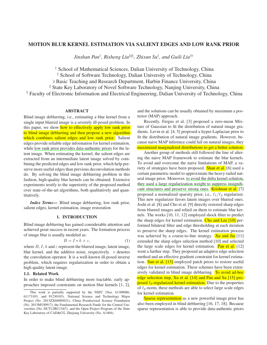
(a)
(b)
(c)
(d)
Fig. 1. The effectiveness of the proposed intermediate latent
image restoration model (3). (a) Blurred image and kernel.
(b) ∇S map visualized using Poisson reconstruction. (c) Re-
sult without the second term in model (3). (d) Result with
model (3). The red boxes shown in (d) contains some sharp
edges.
is defined as
LR(I, L) =
RiI − Li2
F + λLi∗,
(4)
i
, Ii2
where Li denotes the restored image patches with low rank
n×N is the i-
property and RiI = [Ii1
th set of similar image patches extracted from the image I,
which can be obtained by k-Nearest-Neighbor method ac-
cording to [21]. We explain each term of model (3) in detail
as follows.
] ∈ R
, . . . , IiN
1. The first term is the reconstruction error constraint
which ensures the recovered image should be consis-
tent with the input image with respect to the estimated
degradation model.
2. The second term encourages the gradient of I to be sim-
ilar to the salient edges ∇S, which is able to preserve
sharp edges in the recovered latent image.
3. The third term uses low rank prior to provide a data-
authentic prior for the latent image.
Discussion: It is noted that the works [21, 22] also employed
low rank prior to restore images. However, our model is
different from [21, 22]. Our goal is mainly to recover the
sharp edges. Thus, the edge-preserving term (i.e., the sec-
ond term in model (3)) is used. This is the main difference
from [21, 22].
Figure 1 shows comparison results which demonstrate the
effectiveness of our model (3). We note that our estimated
result shown in Figure 1(d) contains more sharp edges which
will provide more useful data for kernel estimation.
2.2. Kernel Estimation via Salient Edges
In order to avoid the delta kernel solution and get a better ker-
nel estimate, most iterative deblurring methods [10, 11] are
carefully designed to select sharp edges for kernel estimation.
Recent work [12] proposes an edge selection method based
on an adaptive Total Variation (TV) model, which has been
proven to be effective in practice. To increase the robustness
of kernel estimation, we adopt the edge selection method [12]
to select the salient edges for kernel estimation. The compu-
tation is as follows.
�
First, we extract the main structures from the intermediate
image I by
min
Is
x
1
2θω(x)
(Is(x) − I(x))2,
where ω(x) = exp(−(r(x))0.8) and r(x) is defined as
∇Is(x)2 +
y∈Nh(x) ∇B(y)2 + 0.5
y∈Nh(x) ∇B(y)2
in which Nh(x) is an h × h window centered at pixel x.
r(x) =
,
Second, we compute an image ˜Is by a shock filter [23]:
= −sign( ˜Is)∇ ˜Is2,
∂ ˜Is
∂t
˜Is|t=0 = Is,
Finally, the salient edges which are used for kernel esti-
mation can be obtained by
∇S = ∇ ˜Is H(∇ ˜Is2, t),
(8)
where denotes the pixel-wise multiplication operator, t is a
threshold, and H(∇ ˜Is2, t) is defined as
H(∇ ˜Is, t) =
1,
0,
∇ ˜Is2 t,
otherwise.
Based on the above considerations, our kernel estimation
model is defined as
min
s.t. k(x) ≥ 0,
∇S ∗ k − ∇B2
k
2 + γk2
2,
k(x) = 1.
x
3. OPTIMIZATION
Intermediate Latent
In this section, we provide more details on solving interme-
diate latent image estimation model (3) and kernel estimation
model (10).
3.1. Optimization for
Restoration
Minimizing model (3) involves simultaneously computing
two variables: I and L, which is computationally challeng-
ing. We employ the alternating minimization scheme, which
is widely adopted when dealing with multiple optimization
variables. Following this optimization framework, we address
each of the optimization variable separately and present an
overall efficient optimization algorithm.
Image
3.1.1. Intermediate latent image I updating
With L fixed, the problem for updating intermediate latent
image I is as
min
I∗k−B2
2 +β∇I−∇S2
2. (11)
2 +τ
I
It is a least squared problem and its closed form solution can
be obtained by using Fast Fourier Transform (FFT):
I = F−1
F(k)F(B) +βF 2 + τF(
F(k)F(k) +βF 1 + τF(
i Li)
i Ri)
i RT
i RT
(12)
,
i
RiI−Li2
(5)
(6)
(7)
(9)
(10)
where F(·) and F−1(·) denote the FFT and inverse FFT, re-
spectively, F(·) is the complex conjugate operator, F1 =
F(∂x)F(∂x) + F(∂y)F(∂y), and F2 = F(∂x)F(∂xS) +
F(∂y)F(∂yS).
3.1.2. Low rank part L updating
With I fixed, the problem for updating L is
RiI − Li2
F + λLi∗,
(13)
i
τ
min
L
which is a standard low-rank approximation problem [24].
Thus, its closed form solution can be obtained by
where UiΣiV T
i
as
Sλ/(2τ )[x] =
i
,
Li = UiSλ/(2τ )[Σi]V T
(14)
is the SVD of RiI and Sλ/(2τ )[x] is defined
⎧⎨
⎩ x − λ/(2τ ),
x > λ/(2τ ),
x < −λ/(2τ ),
otherwise.
x + λ/(2τ ),
0,
(15)
To increase the accuracy of L, we adopt the similar strategy
proposed by [21] to estimate L.
Based on above analysis, our alternating minimization al-
gorithm for the intermediate latent image restoration is sum-
marized in Algorithm 1.
Algorithm 1 Intermediate Latent Image Restoration
Input: Blur image B, blur kernel k, and salient edges ∇S
I ← B.
for i = 1 → 3 do
Estimate L according to (13).
Estimate I according to (11).
end for
Output: Intermediate latent image I.
3.2. Optimization for Kernel Estimation
By writing convolution as matrix multiplication, model (10)
can be written as
V T
k (AT
x Ax + AT
min
Vk
s.t. Vk 0, 1T Vk = 1,
y Ay + γ)Vk − 2(AT
x VBx + AT
y VBy)T Vk,
(16)
where Ax and Ay denote the Toeplitz matrices form of ∂xS
and ∂yS w.r.t k, respectively. VBx, VBy, and Vk denote
the vector form of ∂xB, ∂yB, and k, respectively. 1T =
[1, 1, . . . , 1] has the same size to Vk. Note that model (16)
is a quadratic programming. Thus, the global solution can
be obtained. We employ the dual active-set method to solve
model (16).
Finally, to increase the accuracy of kernel estimation, we
adopt the iterative coarse-to-fine optimization framework that
is commonly used in recent methods [10, 11, 12, 14, 13]. Al-
gorithm 2 presents the main steps in one image level.
�
Algorithm 2 The Proposed Kernel Estimation Algorithm
Input: Blur image B.
Initialize I and k from the previous coarser level.
for j = 1 → 5 (iterations at each level) do
Compute ∇S according to (8).
Estimate k according to (16).
Estimate I by Algorithm 1.
Decrease the values of θ and t to include more edges for
kernel estimation.
end for
Output: Blur kernel k.
4. FINAL LATENT IMAGE RESTORATION
The computed intermediate latent image is not the final latent
natural image estimate due to lack of details (see Figure 1
(d)). To obtain a better latent image with finer textures, we
in this paper choose the non-blind deblurring method with a
hyper-Laplacian prior [25] to recover the final latent image,
which is defined as
min
I
I ∗ k − B2
2 + λf (∂xI0.8 + ∂yI0.8).
We empirically set λf = 3e−3 in our experiments.
(17)
5. ANALYSIS ON THE LOW RANK PRIOR IN
KERNEL ESTIMATION
Although many previous approaches (e.g., [10, 11, 12])
mainly focus on extracting salient edges from the interme-
diate latent image for kernel estimation, we note that if the in-
termediate latent image cannot be recovered well, the salient
edges will have detrimental effect on the kernel estimation.
To demonstrate the effectiveness of low rank prior in the ker-
nel estimation, we compare the proposed method with the
commonly used anisotropic TV regularizer that is employed
in [12] and the proposed method without low rank prior (i.e.,
setting τ = 0 in (3)) under the same salient edges selection
strategy. We use the synthetic dataset from [4], which con-
tains 8 blur kernels and 32 blurred images, for comparison.
In Figure 2(a), we plot the cumulative histograms of de-
convolution error ratios in the same way as [4]. We note that
image deblurring without low rank prior is less effective (see
the baby blue bar in Figure 2(a)). On the other hand, image
deblurring with commonly used anisotropic TV method [12]
is still not effective. The comparison results show that low
rank prior is able to provide reliable data for kernel estima-
tion, thereby facilitating kernel estimation. In Figure 2(b), we
choose an example (i.e., the “im02_ker01” test case in the
dataset in [4]) to demonstrate the validity of our kernel esti-
mation algorithm. Sum of Squared Differences Error (SSDE)
is employed to measure the quality of kernel estimates at each
iteration. As can be seen from Figure 2(b), the estimation er-
ror for the blur kernel is decreasing with increasing iterations,
which empirically justifies the effectiveness of the proposed
Algorithm 2. Moreover, the proposed method performs better
at each iteration.
100
90
80
70
60
50
40
30
20
10
0
1.5
2
2.5
3
3.5
4
With anisotropic TV Without low rank prior With low rank prior
(a)
s
e
t
a
m
i
t
s
e
l
e
n
r
e
k
f
o
E
D
S
S
0.017
0.016
0.015
0.014
0.013
0.012
0.011
0.01
0.009
0
With low rank prior
Without low rank prior
With anisotropic TV
15
20
5
10
Iterations
(b)
Fig. 2. The effectiveness of low rank prior in kernel estima-
(a) Quantitative comparison by using cumulative his-
tion.
tograms of error ratios.
(b) Kernel estimation error plot in
terms of SSDE at each iteration.
6. EXPERIMENTAL RESULTS
In this section, we conduct extensive evaluations on the pro-
posed approach. The parameter t determines the number of
salient edges used for kernel estimation, we in this paper
adaptively set its initial value according to [10]. The parame-
ters β, τ, γ, and θ are empirically set to be 5e−5, 1e−2, 1e−2,
and 1, respectively. The choice of these values are based on
the extensive experimental results. The parameter λ is chosen
according to [21]. In the kernel estimation, all color images
are converted to grayscale ones. In the final deconvolution
process, each color channel is separately processed. Our un-
optimized MATLAB implementation takes several minutes to
estimate a 25×25 kernel from a 255×255 image with an Intel
Xeon CPU@2.53GHz and 12GB RAM.
Quantitative Evaluation on the Dataset of [4]: We per-
form quantitative evaluation of our method using the data set
from [4]. For evaluation with each test case, we follow the
method used in [4]. We also use the provided script and non-
blind deconvolution function to generate the results, for fair-
ness. The error ratio proposed by [4] is used to measure the
quality of estimated results. We compare our method with
those of Fergus et al. [3], Shan et al. [6], Cho and Lee [10],
Xu and Jia [11], Levin et al. [5], Krishnan et al. [7], Pan et
al. [12], Xu et al. [14], Zhong et al. [26], and Sun et al. [13].
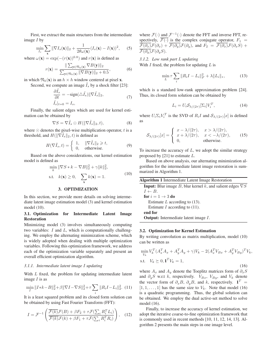
The comparison results are shown in Figure 3. As indicated
in [4], error ratios over 2 will make the result visually im-
plausible. One can see that our method performs the best and
all the error ratio values are below 3. This demonstrates the
effectiveness of the proposed method.
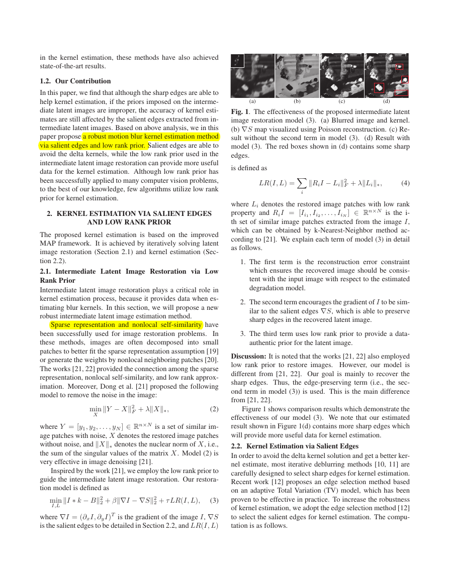
Figure 4 shows one example from the test dataset. As
can be seen from Figure 4, methods of Shan et al. [6], Cho
and Lee [10], Krishnan et al. [7], Pan et al. [12], Zhong et
al. [26] fail to provide reasonable kernel estimates. The de-
blurred results contain some obvious blur. The kernel es-
timates of [11, 14] look better, but the corresponding ker-
nel similarity values are lower than that of our method. In
contrast, the result of our method has the best visual qual-
ity. Moreover, the highest kernel similarity value also shows
that the proposed kernel estimation method outperforms other
state-of-the-art methods.
�
(a) Blurred image
(b) Shan et al. [6]
(c) Cho and Lee [10]
(d) Xu and Jia [11]
(e) Krishnan et al. [7]
(f) Levin et al. [5]
(g) Pan et al. [12]
(h) Xu et al. [14]
(i) Zhong et al. [26]
(j) Our results
Fig. 4. Comparison with state-of-the-art methods on a synthetic example. The kernel similarity values in (b)-(j) are 0.5811,
0.4503, 0.6328, 0.5142, 0.6179, 0.4110, 0.6225, 0.4341, and 0.6504, respectively.
)
%
(
e
t
a
r
s
s
e
c
c
u
S
100
80
60
40
20
0
2
2.5
Ours
Sun et al.
Xu et al.
Zhong et al.
Pan et al.
Levin et al.
Krishnan et al.
Xu and Jia
Cho and Lee
Shan et al.
Fergus et al.
3
3.5
Error ratios
4
4.5
Fig. 3. Quantitative comparison with state-of-the-art methods
on the dataset [4]. Our method performs the best.
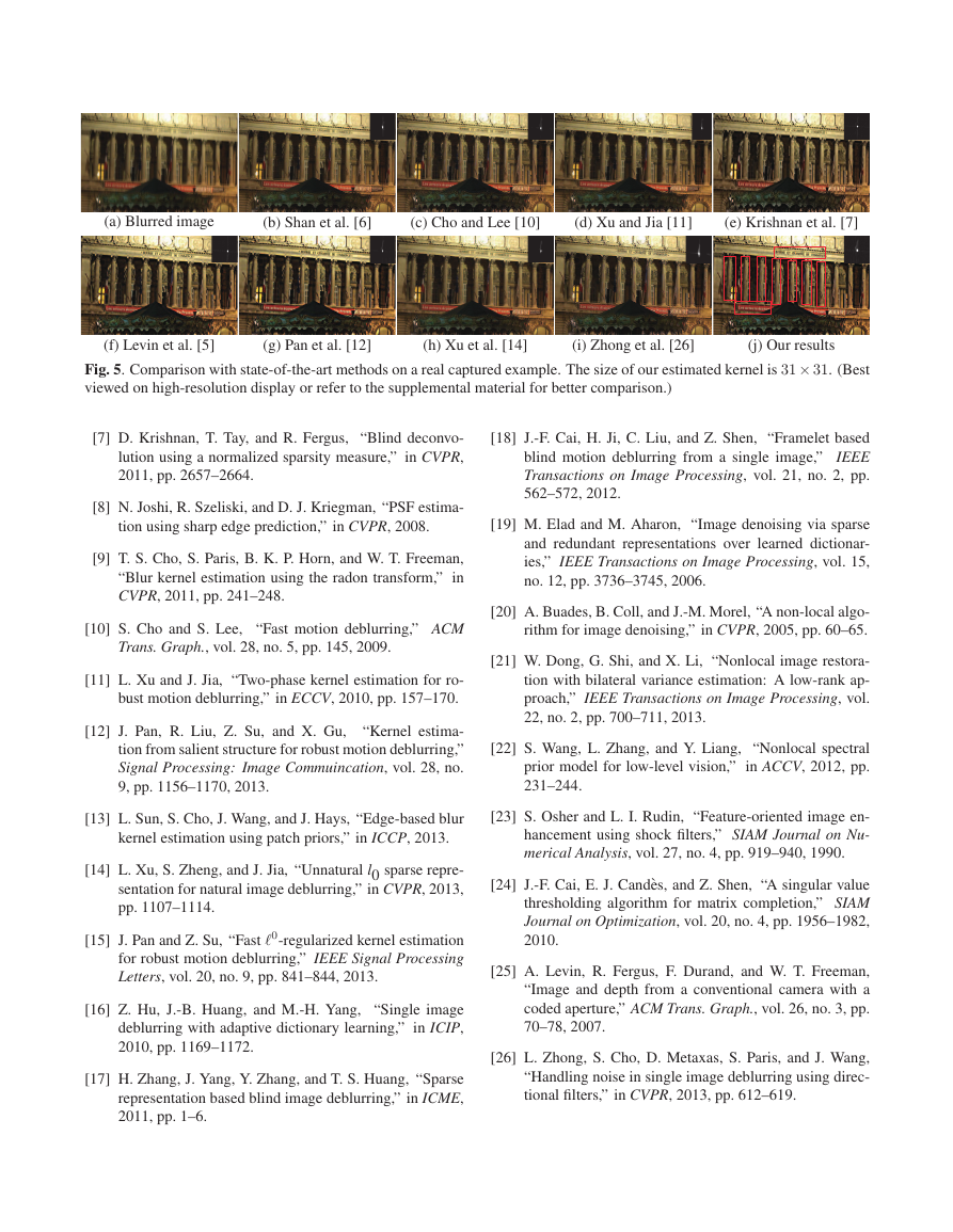
Evaluation on Real Blurred Images: Now we test our
method with some real blurred images. Figure 5 shows an
example that is also presented in [11]. The deblurred results
of [6, 10, 11, 7, 5] still contain some blur. The deblurred result
of Zhong et al. [7] contains some obvious ringing artifacts.
However, the deblurred result from the proposed method con-
tains clearer and finer textures than that of [12] in the red
boxes. More experimental results are included in the supple-
mental material.
7. CONCLUSIONS
In this work, we have presented an effective method for blind
image deblurring. The proposed method combines salient
edges and low rank prior. The salient edges provide reliable
edge information, while the low rank prior offers faithful pri-
ors for the latent image. Their combination greatly improves
the quality of kernel estimation. Both quantitative and qual-
itative evaluations on challenging examples demonstrate that
the proposed method performs favorably against several state-
of-the-art algorithms.
8. REFERENCES
[1] T. Chan and C. Wong, “Total variation blind deconvolu-
tion,” IEEE Transactions on Image Processing, vol. 7,
no. 3, pp. 370–375, 1998.
[2] Y.-L. You and M. Kaveh, “Blind image restoration by
anisotropic regularization,” IEEE Transactions on Im-
age Processing, vol. 8, no. 3, pp. 396–407, 1999.
[3] R. Fergus, B. Singh, A. Hertzmann, S. T. Roweis, and
W. T. Freeman, “Removing camera shake from a single
photograph,” ACM Trans. Graph., vol. 25, no. 3, pp.
787–794, 2006.
[4] A. Levin, Y. Weiss, F. Durand, and W. T. Freeman,
“Understanding and evaluating blind deconvolution al-
gorithms,” in CVPR, 2009, pp. 1964–1971.
[5] A. Levin, Y. Weiss, F. Durand, and W. T. Freeman, “Ef-
ficient marginal likelihood optimization in blind decon-
volution,” in CVPR, 2011, pp. 2657–2664.
[6] Q. Shan, J. Jia, and A. Agarwala, “High-quality motion
deblurring from a single image,” ACM Trans. Graph.,
vol. 27, no. 3, pp. 73, 2008.
�
(a) Blurred image
(b) Shan et al. [6]
(c) Cho and Lee [10]
(d) Xu and Jia [11]
(e) Krishnan et al. [7]
(f) Levin et al. [5]
(g) Pan et al. [12]
Fig. 5. Comparison with state-of-the-art methods on a real captured example. The size of our estimated kernel is 31× 31. (Best
viewed on high-resolution display or refer to the supplemental material for better comparison.)
(h) Xu et al. [14]
(i) Zhong et al. [26]
(j) Our results
[7] D. Krishnan, T. Tay, and R. Fergus, “Blind deconvo-
lution using a normalized sparsity measure,” in CVPR,
2011, pp. 2657–2664.
[8] N. Joshi, R. Szeliski, and D. J. Kriegman, “PSF estima-
tion using sharp edge prediction,” in CVPR, 2008.
[9] T. S. Cho, S. Paris, B. K. P. Horn, and W. T. Freeman,
“Blur kernel estimation using the radon transform,” in
CVPR, 2011, pp. 241–248.
[10] S. Cho and S. Lee, “Fast motion deblurring,” ACM
Trans. Graph., vol. 28, no. 5, pp. 145, 2009.
[11] L. Xu and J. Jia, “Two-phase kernel estimation for ro-
bust motion deblurring,” in ECCV, 2010, pp. 157–170.
[12] J. Pan, R. Liu, Z. Su, and X. Gu,
“Kernel estima-
tion from salient structure for robust motion deblurring,”
Signal Processing: Image Commuincation, vol. 28, no.
9, pp. 1156–1170, 2013.
[13] L. Sun, S. Cho, J. Wang, and J. Hays, “Edge-based blur
kernel estimation using patch priors,” in ICCP, 2013.
[14] L. Xu, S. Zheng, and J. Jia, “Unnatural l0 sparse repre-
sentation for natural image deblurring,” in CVPR, 2013,
pp. 1107–1114.
[15] J. Pan and Z. Su, “Fast 0-regularized kernel estimation
for robust motion deblurring,” IEEE Signal Processing
Letters, vol. 20, no. 9, pp. 841–844, 2013.
[16] Z. Hu, J.-B. Huang, and M.-H. Yang, “Single image
deblurring with adaptive dictionary learning,” in ICIP,
2010, pp. 1169–1172.
[17] H. Zhang, J. Yang, Y. Zhang, and T. S. Huang, “Sparse
representation based blind image deblurring,” in ICME,
2011, pp. 1–6.
[18] J.-F. Cai, H. Ji, C. Liu, and Z. Shen, “Framelet based
blind motion deblurring from a single image,” IEEE
Transactions on Image Processing, vol. 21, no. 2, pp.
562–572, 2012.
[19] M. Elad and M. Aharon, “Image denoising via sparse
and redundant representations over learned dictionar-
ies,” IEEE Transactions on Image Processing, vol. 15,
no. 12, pp. 3736–3745, 2006.
[20] A. Buades, B. Coll, and J.-M. Morel, “A non-local algo-
rithm for image denoising,” in CVPR, 2005, pp. 60–65.
[21] W. Dong, G. Shi, and X. Li, “Nonlocal image restora-
tion with bilateral variance estimation: A low-rank ap-
proach,” IEEE Transactions on Image Processing, vol.
22, no. 2, pp. 700–711, 2013.
[22] S. Wang, L. Zhang, and Y. Liang, “Nonlocal spectral
prior model for low-level vision,” in ACCV, 2012, pp.
231–244.
[23] S. Osher and L. I. Rudin, “Feature-oriented image en-
hancement using shock filters,” SIAM Journal on Nu-
merical Analysis, vol. 27, no. 4, pp. 919–940, 1990.
[24] J.-F. Cai, E. J. Cand`es, and Z. Shen, “A singular value
thresholding algorithm for matrix completion,” SIAM
Journal on Optimization, vol. 20, no. 4, pp. 1956–1982,
2010.
[25] A. Levin, R. Fergus, F. Durand, and W. T. Freeman,
“Image and depth from a conventional camera with a
coded aperture,” ACM Trans. Graph., vol. 26, no. 3, pp.
70–78, 2007.
[26] L. Zhong, S. Cho, D. Metaxas, S. Paris, and J. Wang,
“Handling noise in single image deblurring using direc-
tional filters,” in CVPR, 2013, pp. 612–619.
�



 2023年江西萍乡中考道德与法治真题及答案.doc
 2012年重庆南川中考生物真题及答案.doc
 2013年江西师范大学地理学综合及文艺理论基础考研真题.doc
 2020年四川甘孜小升初语文真题及答案I卷.doc
 2020年注册岩土工程师专业基础考试真题及答案.doc
 2023-2024学年福建省厦门市九年级上学期数学月考试题及答案.doc
 2021-2022学年辽宁省沈阳市大东区九年级上学期语文期末试题及答案.doc
 2022-2023学年北京东城区初三第一学期物理期末试卷及答案.doc
 2018上半年江西教师资格初中地理学科知识与教学能力真题及答案.doc
 2012年河北国家公务员申论考试真题及答案-省级.doc
 2020-2021学年江苏省扬州市江都区邵樊片九年级上学期数学第一次质量检测试题及答案.doc
 2022下半年黑龙江教师资格证中学综合素质真题及答案.doc