3
1
0
2
g
u
A
9
1
]
I
A
.
s
c
[
1
v
8
0
0
4
.
8
0
3
1
:
v
i
X
r
a
A Literature Survey of Benchmark Functions For Global
Optimization Problems
Momin Jamil∗†, Xin-She Yang‡ ∗Blekinge Institute of Technology
SE-37179, Karlskrona, Sweden
†Harman International, Cooperate Division
Becker-Goering Str. 16, D-76307 Karlsbad, Germany
E-mail: momin.jamil@harman.com
‡Middlesex University
School of Science and Technology
Hendon Campus, London NW4 4BT, UK
E-mail: xin-she.yang@middlesex.ac.uk
Citation details:
Momin Jamil and Xin-She Yang, A literature survey of benchmark functions for
global optimization problems, Int. Journal of Mathematical Modelling and
Numerical Optimisation, Vol. 4, No. 2, pp. 150–194 (2013).
DOI: 10.1504/IJMMNO.2013.055204
Test functions are important to validate and compare the performance of optimization
algorithms. There have been many test or benchmark functions reported in the literature;
however, there is no standard list or set of benchmark functions.
Ideally, test functions
should have diverse properties so that can be truly useful to test new algorithms in an
unbiased way. For this purpose, we have reviewed and compiled a rich set of 175 bench-
mark functions for unconstrained optimization problems with diverse properties in terms
of modality, separability, and valley landscape. This is by far the most complete set of
functions so far in the literature, and tt can be expected this complete set of functions can
be used for validation of new optimization in the future.
1
Introduction
The test of reliability, efficiency and validation of optimization algorithms is frequently
carried out by using a chosen set of common standard benchmarks or test functions from
the literature. The number of test functions in most papers varied from a few to about
two dozens. Ideally, the test functions used should be diverse and unbiased, however, there
is no agreed set of test functions in the literature. Therefore, the major aim of this paper
is to review and compile the most complete set of test functions that we can find from all
the available literature so that they can be used for future validation and comparison of
optimization algorithms.
For any new optimization, it is essential to validate its performance and compare with
other existing algorithms over a good set of test functions. A common practice followed
by many researches is to compare different algorithms on a large test set, especially when
1
�
the test involves function optimization (Gordon 1993, Whitley 1996). However, it must be
noted that effectiveness of one algorithm against others simply cannot be measured by the
problems that it solves if the the set of problems are too specialized and without diverse
properties. Therefore, in order to evaluate an algorithm, one must identify the kind of
problems where it performs better compared to others. This helps in characterizing the
type of problems for which an algorithm is suitable. This is only possible if the test suite is
large enough to include a wide variety of problems, such as unimodal, multimodal, regular,
irregular, separable, non-separable and multi-dimensional problems.
Many test functions may be scattered in different textbooks, in individual research
articles or at different web sites. Therefore, searching for a single source of test function
with a wide variety of characteristics is a cumbersome and tedious task. The most notable
attempts to assemble global optimization test problems can be found in [4, 7, 8, 15, 20, 29,
28, 32, 33, 52, 64, 65, 66, 74, 77, 78, 82, 83, 84, 86]. Online collections of test problems also
exist, such as the GLOBAL library at the cross-entropy toolbox [18], GAMS World [36]
CUTE [41], global optimization test problems collection by Hedar [43], collection of test
functions [5, 37, 48, 53, 54, 55, 56, 57, 58, 59], a collection of continuous global optimization
test problems COCONUT [61] and a subset of commonly used test functions [88]. This
motivates us to carry out a thorough analysis and compile a comprehensive collection of
unconstrained optimization test problems.
In general, unconstrained problems can be classified into two categories: test functions
and real-world problems. Test functions are artificial problems, and can be used to evaluate
the behavior of an algorithm in sometimes diverse and difficult situations. Artificial prob-
lems may include single global minimum, single or multiple global minima in the presence of
many local minima, long narrow valleys, null-space effects and flat surfaces. These problems
can be easily manipulated and modified to test the algorithms in diverse scenarios. On the
other hand, real-world problems originate from different fields such as physics, chemistry,
engineering, mathematics etc. These problems are hard to manipulate and may contain
complicated algebraic or differential expressions and may require a significant amount of
data to compile. A collection of real-world unstrained optimization problems can be found
in [7, 8].
In this present work, we will focus on the test function benchmarks and their diverse
properties such as modality and separability. A function with more than one local optimum
is called multimodal. These functions are used to test the ability of an algorithm to escape
from any local minimum.
If the exploration process of an algorithm is poorly designed,
then it cannot search the function landscape effectively. This, in turn, leads to an algorithm
getting stuck at a local minimum. Multi-modal functions with many local minima are among
the most difficult class of problems for many algorithms. Functions with flat surfaces pose a
difficulty for the algorithms, since the flatness of the function does not give the algorithm any
information to direct the search process towards the minima (Stepint, Matyas, PowerSum).
Another group of test problems is formulated by separable and non-separable functions.
According to [16], the dimensionality of the search space is an important issue with the
problem. In some functions, the area that contains that global minima are very small, when
compared to the whole search space, such as Easom, Michalewicz (m=10) and Powell. For
problems such as Perm, Kowalik and Schaffer, the global minimum is located very close to
the local minima. If the algorithm cannot keep up the direction changes in the functions
with a narrow curved valley, in case of functions like Beale, Colville, or cannot explore the
search space effectively, in case of function like Pen Holder, Testtube-Holder having multiple
global minima, the algoritm will fail for these kinds of problems. Another problem that
2
�
algorithms may suffer is the scaling problem with many orders of magnitude differences
between the domain and the function hyper-surface [47], such as Goldstein-Price and Trid.
2 Characteristics of Test Functions
The goal of any global optimization (GO) is to find the best possible solutions x∗ from a
set X according to a set of criteria F = {f1, f2,··· fn}. These criteria are called objective
functions expressed in the form of mathematical functions. An objective function is a
mathematical function f : D ⊂ ℜn → ℜ subject to additional constraints. The set D
is referred to as the set of feasible points in a search space. In the case of optimizing a
single criterion f , an optimum is either its maximum or minimum. The global optimization
problems are often defined as minimization problems, however, these problems can be easily
converted to maximization problems by negating f . A general global optimum problem can
be defined as follows:
minimize
f (x)
x
(1)
The true optimal solution of an optimization problem may be a set of x∗ ∈ D of all optimal
points in D, rather than a single minimum or maximum value in some cases. There could
be multiple, even an infinite number of optimal solutions, depending on the domain of
the search space. The tasks of any good global optimization algorithm is to find globally
optimal or at least sub-optimal solutions. The objective functions could be characterized as
continuous, discontinuous, linear, non-linear, convex, non-conxex, unimodal, multimodal,
separable1 and non-separable.
According to [20], it is important to ask the following two questions before start solving
an optimization problem; (i) What aspects of the function landscape make the optimiza-
tion process difficult? (ii) What type of a priori knowledge is most effective for searching
particular types of function landscape? In order to answer these questions, benchmark
functions can be classified in terms of features like modality, basins, valleys, separability
and dimensionality [87].
2.1 Modality
The number of ambiguous peaks in the function landscape corresponds to the modality of a
function. If algorithms encounters these peaks during a search process, there is a tendency
that the algorithm may be trapped in one of such peaks. This will have a negative impact
on the search process, as this can direct the search away from the true optimal solutions.
2.2 Basins
A relatively steep decline surrounding a large area is called a basin. Optimization algorithms
can be easily attracted to such regions. Once in these regions, the search process of an
algorithm is severely hampered. This is due to lack of information to direct the search
process towards the minimum. According to [20], a basin corresponds to the plateau for a
maximization problem, and a problem can have multiple plateaus.
1In this paper, partially separable functions are also considered as separable function
3
�
2.3 Valleys
A valley occurs when a narrow area of little change is surrounded by regions of steep descent
[20]. As with the basins, minimizers are initially attracted to this region. The progress of a
search process of an algorithm may be slowed down considerably on the floor of the valley.
2.4 Separability
The separability is a measure of difficulty of different benchmark functions.
In general,
separable functions are relatively easy to solve, when compared with their inseperable coun-
terpart, because each variable of a function is independent of the other variables. If all the
parameters or variables are independent, then a sequence of n independent optimization
processes can be performed. As a result, each design variable or parameter can be opti-
mized independently. According to [74], the general condition of separability to see if the
function is easy to optimize or not is given as
∂f (x)
∂xi
= g(xi)h(x)
(2)
where g(xi) means any function of xi only and h(x) any function of any x. If this condition
is satisfied, the function is called partially separable and easy to optimize, because solutions
for each xi can be obtained independently of all the other parameters. This separability
condition can be illustrated by the following two examples.
For example, function (f105) is not separable, because it does not satisfy the condition
(2)
∂f105(x1, x2)
∂x1
∂f105(x1, x2)
∂x2
= 400(x2
1 − x2)x1 − 2x1 − 2
= −200(x2
1 − x2)
On the other hand, the sphere function (f137) with two variables can indeed satisfy the
above condition (2) as shown below.
∂f137(x1, x2)
∂x1
= 2x1
∂f137(x1, x2)
∂x2
= 2x2
where h(x) is regarded as 1.
In [16], the formal definition of separability is given as
arg minimize
x1,...,xp
f (x1, ..., xp) = arg minimize
x1
f (x1, ...), ...,
arg minimize
xp
f (..., xp)
(3)
In other words, a function of p variables is called separable, if it can written as a sum
of p functions of just one variable [16]. On the other hand, a function is called non-
separable, if its variables show inter-relation among themselves or are not independent. If
the objective function variables are independent of each other, then the objective functions
can be decomposed into sub-objective functions. Then, each of these sub-objectives involves
only one decision variable, while treating all the others as constant and can be expressed as
4
�
f (x1, x2,··· , xp) =
fi(xi)
p
Xi=1
(4)
2.5 Dimensionality
The difficulty of a problem generally increases with its dimensionality. According to [87,
90], as the number of parameters or dimension increases, the search space also increases
exponentially. For highly nonlinear problems, this dimensionality may be a significant
barrier for almost all optimization algorithms.
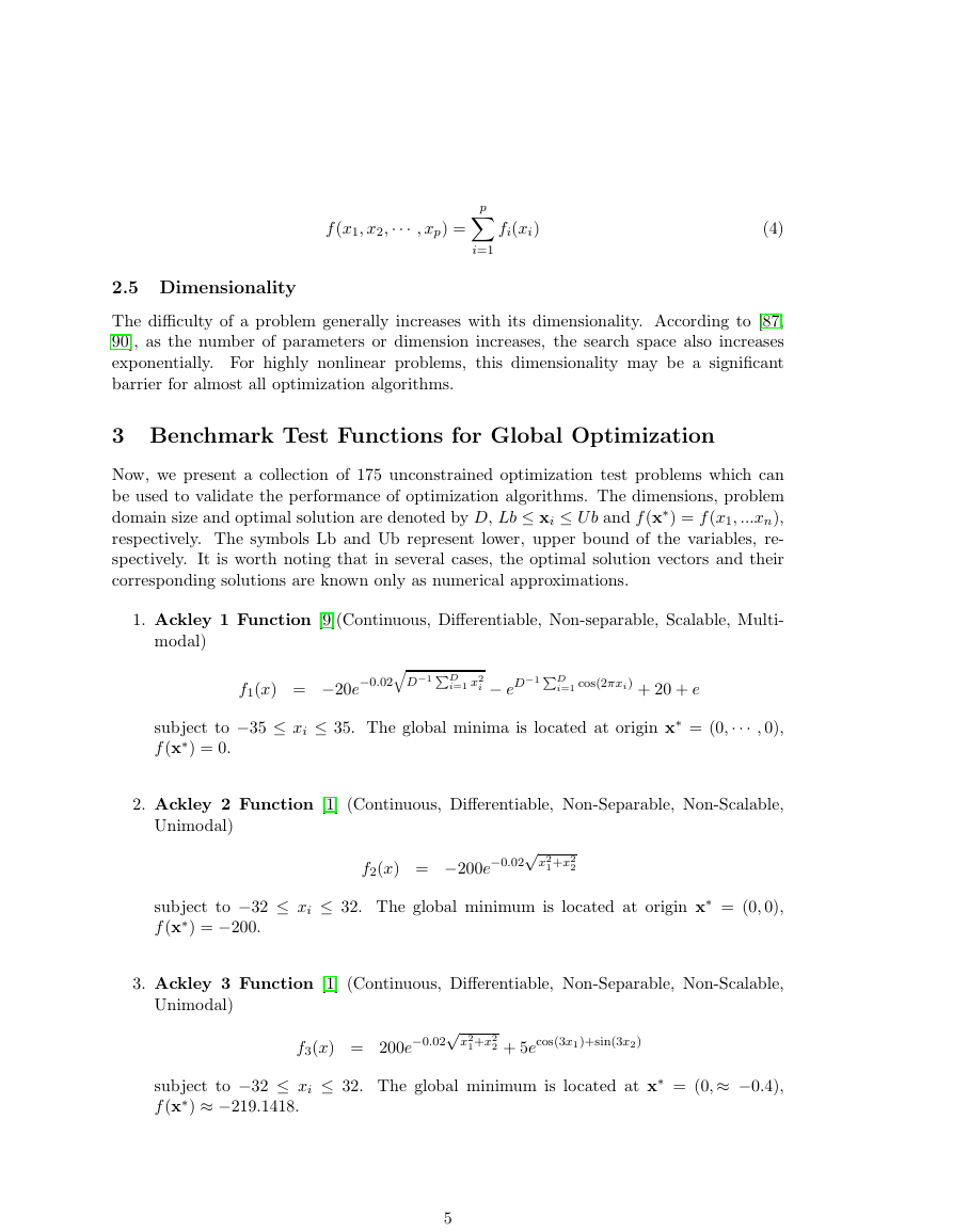
3 Benchmark Test Functions for Global Optimization
Now, we present a collection of 175 unconstrained optimization test problems which can
be used to validate the performance of optimization algorithms. The dimensions, problem
domain size and optimal solution are denoted by D, Lb ≤ xi ≤ U b and f (x∗) = f (x1, ...xn),
respectively. The symbols Lb and Ub represent lower, upper bound of the variables, re-
spectively. It is worth noting that in several cases, the optimal solution vectors and their
corresponding solutions are known only as numerical approximations.
1. Ackley 1 Function [9](Continuous, Differentiable, Non-separable, Scalable, Multi-
modal)
f1(x) = −20e−0.02qD−1 PD
i=1 x2
i − eD−1 PD
i=1 cos(2πxi) + 20 + e
subject to −35 ≤ xi ≤ 35. The global minima is located at origin x∗ = (0,··· , 0),
f (x∗) = 0.
2. Ackley 2 Function [1] (Continuous, Differentiable, Non-Separable, Non-Scalable,
Unimodal)
f2(x) = −200e−0.02√x2
1+x2
2
subject to −32 ≤ xi ≤ 32. The global minimum is located at origin x∗ = (0, 0),
f (x∗) = −200.
3. Ackley 3 Function [1] (Continuous, Differentiable, Non-Separable, Non-Scalable,
Unimodal)
f3(x) = 200e−0.02√x2
1+x2
2 + 5ecos(3x1)+sin(3x2)
subject to −32 ≤ xi ≤ 32. The global minimum is located at x∗ = (0,≈ −0.4),
f (x∗) ≈ −219.1418.
5
�
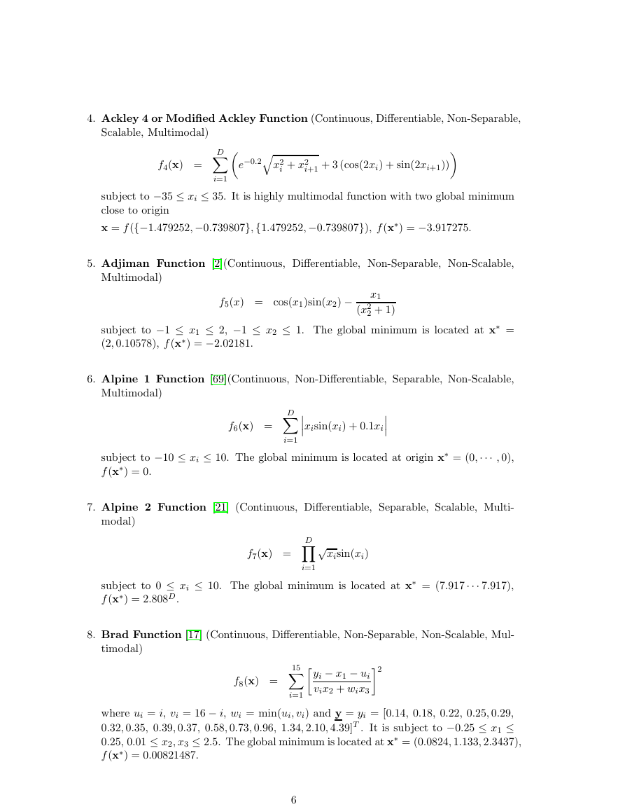
4. Ackley 4 or Modified Ackley Function (Continuous, Differentiable, Non-Separable,
Scalable, Multimodal)
f4(x) =
D
Xi=1e−0.2qx2
i + x2
i+1 + 3 (cos(2xi) + sin(2xi+1))
subject to −35 ≤ xi ≤ 35. It is highly multimodal function with two global minimum
close to origin
x = f ({−1.479252,−0.739807},{1.479252, −0.739807}), f (x∗) = −3.917275.
5. Adjiman Function [2](Continuous, Differentiable, Non-Separable, Non-Scalable,
Multimodal)
f5(x) = cos(x1)sin(x2) −
x1
2 + 1)
(x2
subject to −1 ≤ x1 ≤ 2, −1 ≤ x2 ≤ 1. The global minimum is located at x∗ =
(2, 0.10578), f (x∗) = −2.02181.
6. Alpine 1 Function [69](Continuous, Non-Differentiable, Separable, Non-Scalable,
Multimodal)
f6(x) =
D
xisin(xi) + 0.1xi
Xi=1
subject to −10 ≤ xi ≤ 10. The global minimum is located at origin x∗ = (0,··· , 0),
f (x∗) = 0.
7. Alpine 2 Function [21] (Continuous, Differentiable, Separable, Scalable, Multi-
modal)
f7(x) =
√xisin(xi)
D
Yi=1
subject to 0 ≤ xi ≤ 10. The global minimum is located at x∗ = (7.917··· 7.917),
f (x∗) = 2.808D.
8. Brad Function [17] (Continuous, Differentiable, Non-Separable, Non-Scalable, Mul-
timodal)
f8(x) =
15
vix2 + wix32
Xi=1 yi − x1 − ui
where ui = i, vi = 16 − i, wi = min(ui, vi) and y = yi = [0.14, 0.18, 0.22, 0.25, 0.29,
0.32, 0.35, 0.39, 0.37, 0.58, 0.73, 0.96, 1.34, 2.10, 4.39]T . It is subject to −0.25 ≤ x1 ≤
0.25, 0.01 ≤ x2, x3 ≤ 2.5. The global minimum is located at x∗ = (0.0824, 1.133, 2.3437),
f (x∗) = 0.00821487.
6
�
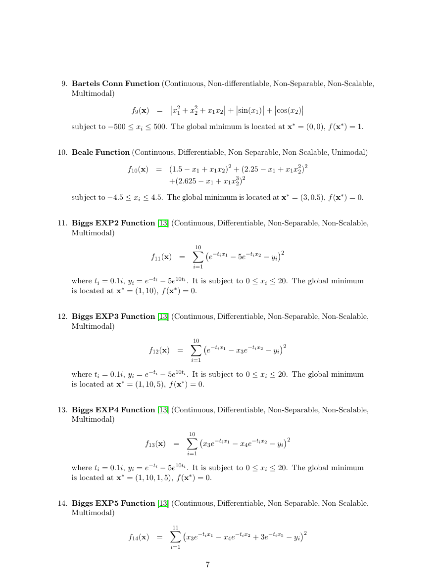
9. Bartels Conn Function (Continuous, Non-differentiable, Non-Separable, Non-Scalable,
Multimodal)
subject to −500 ≤ xi ≤ 500. The global minimum is located at x∗ = (0, 0), f (x∗) = 1.
2 + x1x2 +sin(x1) +cos(x2)
1 + x2
f9(x) = x2
10. Beale Function (Continuous, Differentiable, Non-Separable, Non-Scalable, Unimodal)
2)2
f10(x) = (1.5 − x1 + x1x2)2 + (2.25 − x1 + x1x2
2)2
+(2.625 − x1 + x1x3
subject to −4.5 ≤ xi ≤ 4.5. The global minimum is located at x∗ = (3, 0.5), f (x∗) = 0.
11. Biggs EXP2 Function [13] (Continuous, Differentiable, Non-Separable, Non-Scalable,
Multimodal)
f11(x) =
10
Xi=1e−tix1 − 5e−tix2 − yi2
where ti = 0.1i, yi = e−ti − 5e10ti . It is subject to 0 ≤ xi ≤ 20. The global minimum
is located at x∗ = (1, 10), f (x∗) = 0.
12. Biggs EXP3 Function [13] (Continuous, Differentiable, Non-Separable, Non-Scalable,
Multimodal)
f12(x) =
10
Xi=1e−tix1 − x3e−tix2 − yi2
where ti = 0.1i, yi = e−ti − 5e10ti . It is subject to 0 ≤ xi ≤ 20. The global minimum
is located at x∗ = (1, 10, 5), f (x∗) = 0.
13. Biggs EXP4 Function [13] (Continuous, Differentiable, Non-Separable, Non-Scalable,
Multimodal)
f13(x) =
10
Xi=1x3e−tix1 − x4e−tix2 − yi2
where ti = 0.1i, yi = e−ti − 5e10ti . It is subject to 0 ≤ xi ≤ 20. The global minimum
is located at x∗ = (1, 10, 1, 5), f (x∗) = 0.
14. Biggs EXP5 Function [13] (Continuous, Differentiable, Non-Separable, Non-Scalable,
Multimodal)
f14(x) =
11
Xi=1x3e−tix1 − x4e−tix2 + 3e−tix5 − yi2
7
�
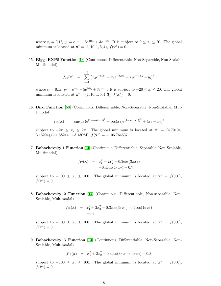
where ti = 0.1i, yi = e−ti − 5e10ti + 3e−4ti . It is subject to 0 ≤ xi ≤ 20. The global
minimum is located at x∗ = (1, 10, 1, 5, 4), f (x∗) = 0.
15. Biggs EXP5 Function [13] (Continuous, Differentiable, Non-Separable, Non-Scalable,
Multimodal)
f15(x) =
13
Xi=1x3e−tix1 − x4e−tix2 + x6e−tix5 − yi2
where ti = 0.1i, yi = e−ti − 5e10ti + 3e−4ti. It is subject to −20 ≤ xi ≤ 20. The global
minimum is located at x∗ = (1, 10, 1, 5, 4, 3), f (x∗) = 0.
16. Bird Function [58] (Continuous, Differentiable, Non-Separable, Non-Scalable, Mul-
timodal)
f16(x) = sin(x1)e(1−cos(x2))2
+ cos(x2)e(1−sin(x1))2
+ (x1 − x2)2
subject to −2π ≤ xi ≤ 2π. The global minimum is located at x∗ = (4.70104,
3.15294),(−1.58214, −3.13024), f (x∗) = −106.764537.
17. Bohachevsky 1 Function [14] (Continuous, Differentiable, Separable, Non-Scalable,
Multimodal)
f17(x) = x2
2 − 0.3cos(3πx1)
1 + 2x2
−0.4cos(4πx2) + 0.7
subject to −100 ≤ xi ≤ 100. The global minimum is located at x∗ = f (0, 0),
f (x∗) = 0.
18. Bohachevsky 2 Function [14] (Continuous, Differentiable, Non-separable, Non-
Scalable, Multimodal)
f18(x) = x2
1 + 2x2
+0.3
2 − 0.3cos(3πx1) · 0.4cos(4πx2)
subject to −100 ≤ xi ≤ 100. The global minimum is located at x∗ = f (0, 0),
f (x∗) = 0.
19. Bohachevsky 3 Function [14] (Continuous, Differentiable, Non-Separable, Non-
Scalable, Multimodal)
f19(x) = x2
1 + 2x2
2 − 0.3cos(3πx1 + 4πx2) + 0.3
subject to −100 ≤ xi ≤ 100. The global minimum is located at x∗ = f (0, 0),
f (x∗) = 0.
8
�


 2023年江西萍乡中考道德与法治真题及答案.doc
 2012年重庆南川中考生物真题及答案.doc
 2013年江西师范大学地理学综合及文艺理论基础考研真题.doc
 2020年四川甘孜小升初语文真题及答案I卷.doc
 2020年注册岩土工程师专业基础考试真题及答案.doc
 2023-2024学年福建省厦门市九年级上学期数学月考试题及答案.doc
 2021-2022学年辽宁省沈阳市大东区九年级上学期语文期末试题及答案.doc
 2022-2023学年北京东城区初三第一学期物理期末试卷及答案.doc
 2018上半年江西教师资格初中地理学科知识与教学能力真题及答案.doc
 2012年河北国家公务员申论考试真题及答案-省级.doc
 2020-2021学年江苏省扬州市江都区邵樊片九年级上学期数学第一次质量检测试题及答案.doc
 2022下半年黑龙江教师资格证中学综合素质真题及答案.doc