Log-linear models
and
conditional random fields
Notes for a tutorial at CIKM’08
Charles Elkan
elkan@cs.ucsd.edu
October 20, 2008
�
Contents
1 Likelihood and logistic regression
1.1 Principle of maximum likelihood . . . . . . . . . . . . . . . . . .
1.2 Maximum likelihood for Bernoulli distributions . . . . . . . . . .
1.3 Conditional likelihood . . . . . . . . . . . . . . . . . . . . . . .
1.4 Logistic regression . . . . . . . . . . . . . . . . . . . . . . . . .
2 Stochastic gradient training
2.1 Logistic regression gradient . . . . . . . . . . . . . . . . . . . . .
2.2 Gradient ascent, one example at a time . . . . . . . . . . . . . . .
2.3 Properties of stochastic gradient training . . . . . . . . . . . . . .
3 Log-linear models
3.1 The general log-linear model
. . . . . . . . . . . . . . . . . . . .
3.2 Feature functions . . . . . . . . . . . . . . . . . . . . . . . . . .
4 Conditional random fields
4.1 A typical CRF application . . . . . . . . . . . . . . . . . . . . .
4.2 Linear-chain CRFs in general . . . . . . . . . . . . . . . . . . . .
4.3
. . . . . . . . . . . .
4.4 Training CRFs by stochastic gradient ascent . . . . . . . . . . . .
Inference algorithms for linear-chain CRFs
5 Alternative CRF training methods
5.1 The Collins perceptron . . . . . . . . . . . . . . . . . . . . . . .
5.2 Gibbs sampling .
. . . . . . . . . . . . . . . . . . . . . . . . . .
5.3 Contrastive divergence . . . . . . . . . . . . . . . . . . . . . . .
6 Tutorials and selected papers
2
2
3
4
4
6
6
7
8
10
10
11
12
12
13
15
17
20
20
21
23
24
1
�
Chapter 1
Likelihood and logistic regression
Logistic regression is the simplest example of a log-linear model, so this section
examines logistic regression in detail. All log-linear models are based on the idea
of maximizing likelihood, so we shall discuss that general idea first of all.
1.1 Principle of maximum likelihood
Consider a family of probability distributions defined by a set of parameters θ.
The distributions may be either probability mass functions (pmfs) or probability
density functions (pdfs). Suppose we have a random sample drawn from a fixed
but unknown member of this family. The random sample is a training set of n ex-
amples x1 to xn. We assume that the examples are independent so the probability
of the set is the product of the probabilities of the individual examples:
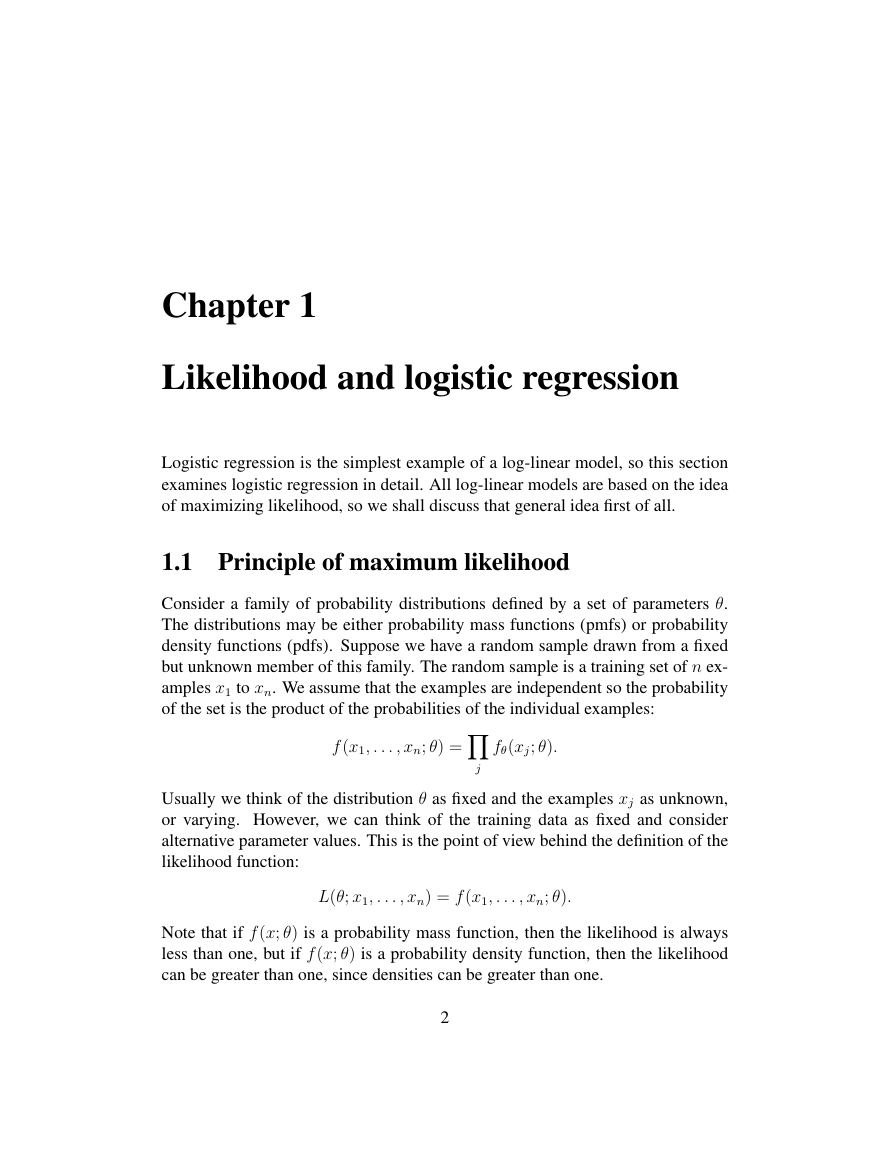
Y
f (x1, . . . , xn; θ) =
fθ(xj; θ).
j
Usually we think of the distribution θ as fixed and the examples xj as unknown,
or varying. However, we can think of the training data as fixed and consider
alternative parameter values. This is the point of view behind the definition of the
likelihood function:
L(θ; x1, . . . , xn) = f (x1, . . . , xn; θ).
Note that if f (x; θ) is a probability mass function, then the likelihood is always
less than one, but if f (x; θ) is a probability density function, then the likelihood
can be greater than one, since densities can be greater than one.
2
�
The principle of maximum likelihood says that we should use as our model
the distribution f (·; ˆθ) that gives the greatest possible probability to the training
data. Formally,
ˆθ = argmaxθL(θ; x1, . . . , xn).
This value ˆθ is called the maximum likelihood estimator (MLE) of θ. Note that in
general each xj is a vector of values, and θ is a vector of real-valued parameters.
For example, for a Gaussian distribution θ = hµ, σ2i.
Notational note: In the expression p(y|x; β) the semicolon indicates that β is
a parameter, not a random variable that is being conditioned on, even though it
is to the right of the vertical bar. Viewed as a mapping, this expression is simply
a function of three arguments. Viewed as a probability, it is a property of two
random variables. In a Bayesian framework, parameters are also viewed as ran-
dom variables, and one can write expressions such as p(β|x). We are not doing a
Bayesian analysis, so we indicate that β is not a random variable.
1.2 Maximum likelihood for Bernoulli distributions
As a first example of finding a maximum likelihood estimator, consider the pa-
rameter of a Bernoulli distribution. A random variable with this distribution is a
formalization of a coin toss. The value of the random variable is 1 with probability
θ and 0 with probability 1 − θ. Let X be a Bernoulli random variable. We have
P (X = x) =
θ if x = 1
1 − θ if x = 0
.
For mathematical convenience write this as
P (X = x) = θx(1 − θ)1−x.
Suppose the training data are x1 through xn where each xj ∈ {0, 1}. We maximize
the likelihood function
where h =P
L(θ; x1, . . . , xn) = f (x1, . . . , xn; θ) = θh(1 − θ)n−h
i xi. The maximization is over the possible values 0 ≤ θ ≤ 1.
We can do the maximization by setting the derivative with respect to θ equal
to zero. The derivative is
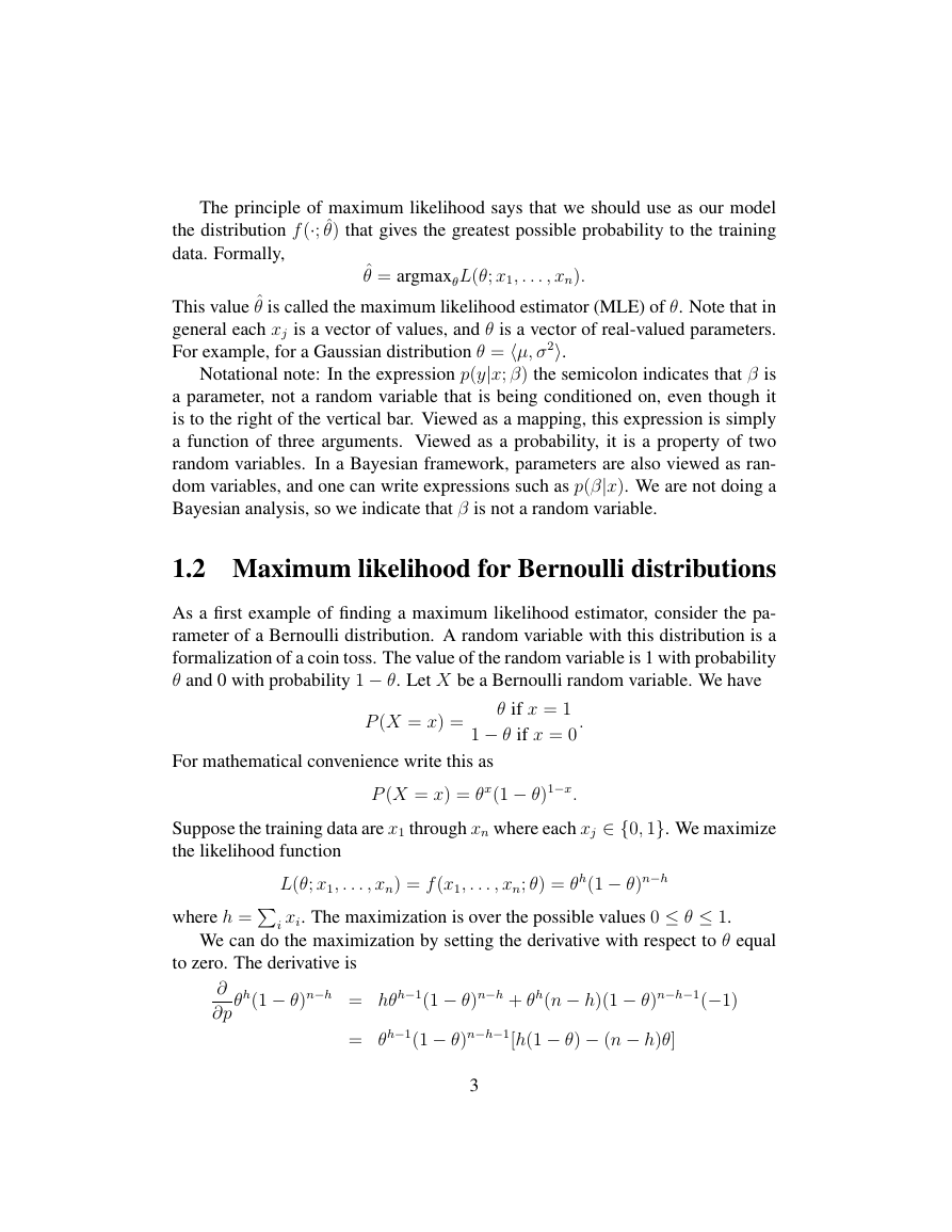
∂
∂p
θh(1 − θ)n−h = hθh−1(1 − θ)n−h + θh(n − h)(1 − θ)n−h−1(−1)
= θh−1(1 − θ)n−h−1[h(1 − θ) − (n − h)θ]
3
�
which has solutions θ = 0, θ = 1, and θ = h/n. The solution which is a maximum
is clearly θ = h/n while θ = 0 and θ = 1 are minima. So we have the maximum
likelihood estimate ˆθMLE = h/n.
The log likelihood function is simply the logarithm of the likelihood function.
Because logarithm is a monotonic strictly increasing function, maximizing the log
likelihood is precisely equivalent to maximizing the likelihood, or to minimizing
the negative log likelihood.
1.3 Conditional likelihood
An important extension of the idea of likelihood is conditional likelihood. The
conditional likelihood of θ given data x and y is L(θ; y|x) = f (y|x; θ). Intuitively,
y follows a probability distribution that is different for different x, but x itself is
never unknown, so there is no need to have a probabilistic model of it. Technically,
for each x there is a different distribution f (y|x; θ) of y, but all these distributions
share the same parameters θ.
Given training data consisting of hxi, yii pairs, the principle of maximum con-
ditional likelihood says to choose a parameter estimate ˆθ that maximizes the prod-
i f (yi|xi; θ). Note that we do not need to assume that the xi are independent
in order to justify the conditional likelihood being a product; we just need to as-
sume that the yi are independent conditional on the xi. For any specific value of
x, ˆθ can be used to predict values for y; we assume that we never want to predict
values of x.
uctQ
1.4 Logistic regression
If y is a binary outcome and x is a real-valued vector, then the conditional model
p = p(y|x; α, β) =
1 + exp−[α +Pd
1
j=1 βjxj]
is called logistic regression. We use j to index over the feature values x1 to xd of
a single example of dimensionality d, since we use i below to index over training
examples 1 to n.
The logistic regression model is easier to understand in the form
X
j
βjxj.
log
p
1 − p
= α +
4
�
linear expression of the form α +P
The ratio p/(1 − p) is called the odds of the event y given x, and log[p/(1 − p)]
is called the log odds. Since probabilities range between 0 and 1, odds range
between 0 and +∞ and log odds range unboundedly between −∞ and +∞. A
j βjxj can also take unbounded values, so
it is reasonable to use a linear expression as a model for log odds, but not as a
model for odds or for probabilities. Essentially, logistic regression is the simplest
possible model for a random yes/no outcome that depends linearly on predictors
x1 to xd.
For each feature j, exp(βjxj) is a multiplicative scaling factor on the odds
p/(1 − p). If the predictor xj is binary, then exp(βj) is the extra odds of having
the outcome y = 1 when xj = 1, compared to when xj = 0.
Note that it is acceptable, and indeed often beneficial, to include a large num-
ber of features in a logistic regression model. Some features may be derived,
i.e. computed as deterministic functions of other features. One great advantage
of logistic regression in comparison to other classifiers is that the training process
will find optimal coefficients for features regardless of whether the features are
correlated. Other learning methods, in particular naive Bayes, do not work well
when the feature values of training or test examples are correlated.
A second major advantage of logistic regression is that it gives well-calibrated
probabilities. The numerical values p(y = 1|x) given by a logistic regression
model are not just scores where a larger score means that the example x is more
likely to have label y = 1; they are meaningful conditional probabilities. This
implies that given a set of n test examples with numerical predictions v1 to vn,
i=1 vi,
the number of examples in the set that are truly positive will be close toPn
whatever this sum is.
Last but not least, a third major advantage of logistic regression is that it is not
sensitive to unbalanced training data. What this means is that even if one class (ei-
ther the positive or negative examples) is much larger than the other (correspond-
ingly, the negative or positive examples), logistic regression training encounters
no difficulties and the final classifier will still be well-calibrated. The conditional
probabilities predicted by the trained classifier will range below and above the
base rate, i.e. the unconditional probability p(y = 1).
5
�
Chapter 2
Stochastic gradient training
All training algorithms for log-linear models are based on the gradient of the con-
ditional likelihood function, or on a closely related idea. The simplest of these
training algorithms, which are often the fastest and most useful in practice, use
the gradient computed from one training example at a time. These algorithms are
called stochastic gradient methods.
2.1 Logistic regression gradient
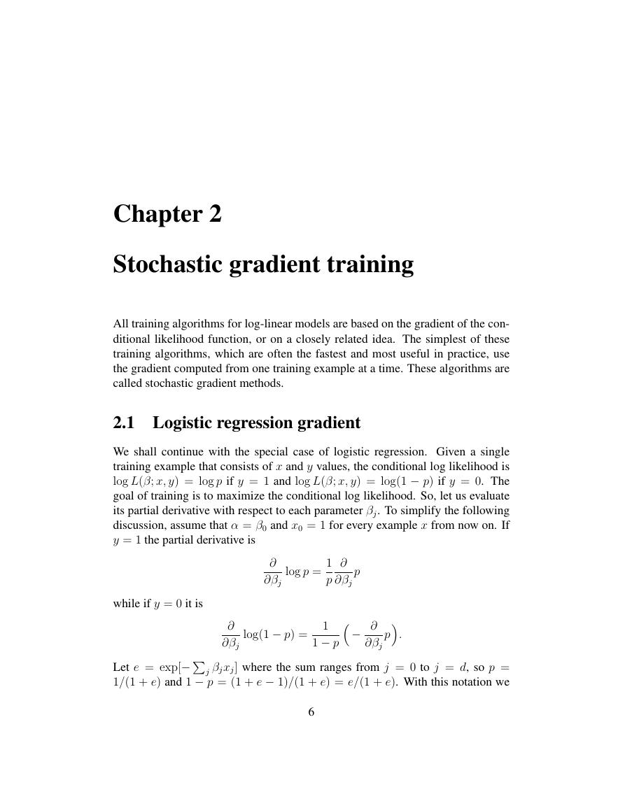
We shall continue with the special case of logistic regression. Given a single
training example that consists of x and y values, the conditional log likelihood is
log L(β; x, y) = log p if y = 1 and log L(β; x, y) = log(1 − p) if y = 0. The
goal of training is to maximize the conditional log likelihood. So, let us evaluate
its partial derivative with respect to each parameter βj. To simplify the following
discussion, assume that α = β0 and x0 = 1 for every example x from now on. If
y = 1 the partial derivative is
∂
∂βj
log p =
1
p
while if y = 0 it is
∂
∂βj
p
Let e = exp[−P
∂
∂βj
log(1 − p) =
1
1 − p
j βjxj] where the sum ranges from j = 0 to j = d, so p =
1/(1 + e) and 1 − p = (1 + e − 1)/(1 + e) = e/(1 + e). With this notation we
− ∂
.
p
∂βj
6
�
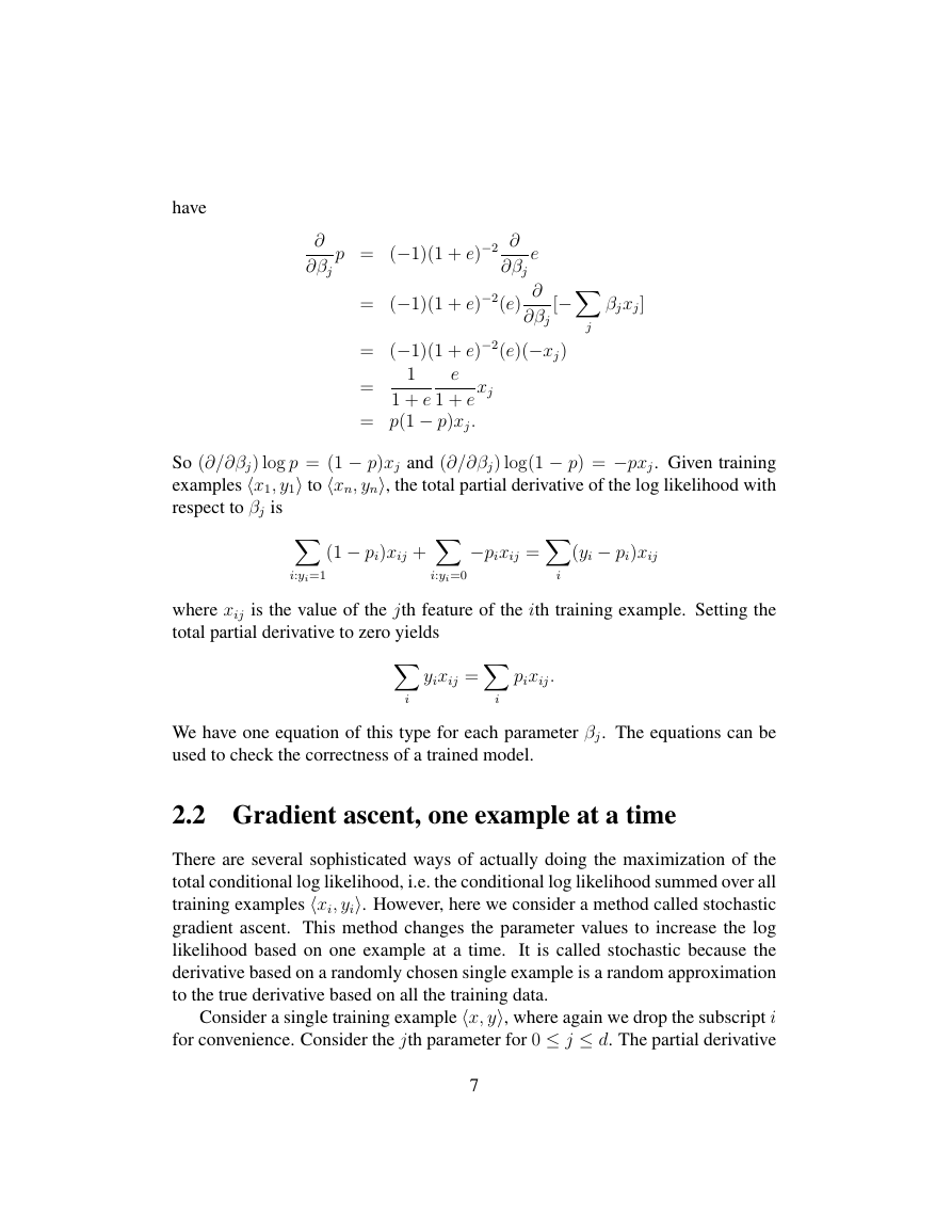
have
∂
∂βj
[−X
j
e
p = (−1)(1 + e)−2 ∂
∂βj
= (−1)(1 + e)−2(e)
= (−1)(1 + e)−2(e)(−xj)
e
=
1 + e
= p(1 − p)xj.
∂
∂βj
1 + e
xj
1
βjxj]
So (∂/∂βj) log p = (1 − p)xj and (∂/∂βj) log(1 − p) = −pxj. Given training
examples hx1, y1i to hxn, yni, the total partial derivative of the log likelihood with
X
X
respect to βj is X
(1 − pi)xij +
−pixij =
(yi − pi)xij
i:yi=1
i:yi=0
i
where xij is the value of the jth feature of the ith training example. Setting the
total partial derivative to zero yieldsX
X
yixij =
pixij.
i
i
We have one equation of this type for each parameter βj. The equations can be
used to check the correctness of a trained model.
2.2 Gradient ascent, one example at a time
There are several sophisticated ways of actually doing the maximization of the
total conditional log likelihood, i.e. the conditional log likelihood summed over all
training examples hxi, yii. However, here we consider a method called stochastic
gradient ascent. This method changes the parameter values to increase the log
likelihood based on one example at a time.
It is called stochastic because the
derivative based on a randomly chosen single example is a random approximation
to the true derivative based on all the training data.
Consider a single training example hx, yi, where again we drop the subscript i
for convenience. Consider the jth parameter for 0 ≤ j ≤ d. The partial derivative
7
�




 2023年江西萍乡中考道德与法治真题及答案.doc
 2012年重庆南川中考生物真题及答案.doc
 2013年江西师范大学地理学综合及文艺理论基础考研真题.doc
 2020年四川甘孜小升初语文真题及答案I卷.doc
 2020年注册岩土工程师专业基础考试真题及答案.doc
 2023-2024学年福建省厦门市九年级上学期数学月考试题及答案.doc
 2021-2022学年辽宁省沈阳市大东区九年级上学期语文期末试题及答案.doc
 2022-2023学年北京东城区初三第一学期物理期末试卷及答案.doc
 2018上半年江西教师资格初中地理学科知识与教学能力真题及答案.doc
 2012年河北国家公务员申论考试真题及答案-省级.doc
 2020-2021学年江苏省扬州市江都区邵樊片九年级上学期数学第一次质量检测试题及答案.doc
 2022下半年黑龙江教师资格证中学综合素质真题及答案.doc