CC2431 Location Engine
1 KEYWORDS
• CC2430
• CC2431
INTRODUCTION
2
This document describes
the
location
engine
the CC2431.
CC2431 is a ZigBee system on chip, so it
will be natural to use the location engine in
a ZigBee network. This manual is written
to be as general as possible and will not
describe
specific
considerations.
protocol
implemented
in
any
Application Note AN042
By K. Aamodt
• ZigBee
• Location Engine
The main purposes of this document it to
present some basic aspects of the location
technology, and provide some hints and
tips for easy developing of systems using
the CC2431
location engine. This
document should be read as an extension
to the CC2431 and CC2430 data sheets.
Application Note AN042 (Rev. 1.0)
SWRA095
Page 1 of 20
�
Application Note AN042
Table of Contents
1
2
3
KEYWORDS ................................................................................................................... 1
INTRODUCTION............................................................................................................. 1
LOCATION ENGINE....................................................................................................... 3
NODE TYPES.............................................................................................................. 4
Reference node .................................................................................................................4
Blind Node........................................................................................................................4
THE LOCATION HARDWARE ......................................................................................... 4
Input..................................................................................................................................5
Output...............................................................................................................................5
RECEIVED SIGNAL STRENGTH INDICATOR (RSSI) ................................................. 6
OFFSET..................................................................................................................... 6
LINEARITY.................................................................................................................. 6
THEORETICAL SIGNAL PROPAGATION........................................................................... 7
RSSI – PRACTICAL CONSIDERATIONS ......................................................................... 7
Simple ways to filter the RSSI values................................................................................7
Calculated RSSI vs. measured RSSI .................................................................................8
DIFFERENT PARAMETERS – INFLUENCE ................................................................. 9
A – RSSI VALUE MEASURED ONE METER FROM THE SENDER ...................................... 10
Measuring A ...................................................................................................................10
A versus calculated position...........................................................................................11
N – SIGNAL PROPAGATION COEFFICIENT ................................................................... 12
Measuring n....................................................................................................................13
NUMBER OF REFERENCE NODES ............................................................................... 14
SOFTWARE ALGORITHMS ........................................................................................ 15
SELECTION OF “BEST” REFERENCE NODES................................................................. 15
EXTENSION OF THE COVERED AREA........................................................................... 15
LEVEL/ FLOOR INDICATION ........................................................................................ 16
CONTROL SYSTEM/ CENTRAL ................................................................................. 18
GENERAL INFORMATION .......................................................................................... 19
DOCUMENT HISTORY................................................................................................ 19
IMPORTANT NOTICE .................................................................................................. 20
4.4.1
4.4.2
5.1.1
5.1.2
5.2.1
3.1
3.2
3.1.1
3.1.2
3.2.1
3.2.2
4.1
4.2
4.3
4.4
5.1
5.2
5.3
6.1
6.2
6.3
8.1
4
5
6
7
8
9
Application Note AN042 (Rev. 1.0)
SWRA095
Page 2 of 20
�
Application Note AN042
3 LOCATION ENGINE
The location algorithm used in the CC2431 Location Engine is based on Received Signal
Strength Indicator (RSSI) values. The RSSI value will decrease when the distance increases.
Figure 1: Location Estimation
Figure 1 shows a simplified system for location detection. “Reference node” is a static node
placed at a known position. For simplicity this node knows its own position and can tell other
nodes where it is on request. A reference node does not need to implement the hardware
needed for location detection, it will not perform any calculation at all. A “Blind node” is a node
built with CC2431. This node will collect signals from all reference nodes responding to a
request, read out the respective RSSI values, feed the collected values into the hardware
engine, and afterwards it reads out the calculated position and sends the position information
to a control application.
The minimum data contained in a packet sent from a reference node to a blind node shall be
the reference nodes’ X and Y parameters. The RSSI value is calculated by the receiver, i.e.
the blind node.
The main feature of the location engine is that the location calculation can be performed at
each blind node, hence the algorithm is decentralised. This property reduces the amount of
data transferred in the network, since only the calculated position is transferred, not the data
used to perform the calculation.
To map each location to a distinct place in the natural environment, a two dimensional grid is
used. The directions will, in the following, be denoted X and Y. In all the figures X is defined to
be the horizontal direction and Y the vertical. The CC2431 Location Engine can only handle
two dimensions, but it’s possible to handle a third dimension in software (i.e. to represent
floors in a building). The point named (X, Y) = (0, 0) is located in the upper left corner of the
grid.
Application Note AN042 (Rev. 1.0)
SWRA095
Page 3 of 20
�
3.1 Node types
Application Note AN042
3.1.1 Reference node
A node which has a static location is called a reference node. This node must be configured
with X and Y value that correspond to the physical location.
The main task for a reference node is to provide a “reference” packet that contains X and Y
coordinates to the blind node, also referred to as an anchor node.
Since this node is not using the hardware location engine at all, it is not necessary to use a
CC2431 for the purpose. This means that a reference node can be run on either a CC2430 or
a CC2431. Since CC2430/31 is based on the same transceiver as CC2420, even a CC2420
together with a suitable microcontroller can be used as reference node.
3.1.2 Blind Node
A blind node will communicate with the closest reference nodes, collecting X, Y and RSSI for
each of these nodes, and calculate its position based on the parameter input using the
location engine hardware. Afterwards the calculated position should be sent to a control
station. This control station could be a PC or another node in the system.
A blind node must be using CC2431.
3.2 The location hardware
The location engine utilizes an extremely simple interface seen from the software layer; write
parameters in, wait for the calculation to performed, and read out the calculated position out.
This chapter will discuss the different parameters and how the shall be interpreted.
Figure 2: Location Engine, input and output
Application Note AN042 (Rev. 1.0)
SWRA095
Page 4 of 20
�
Application Note AN042
Input
3.2.1
Table 1 shows all necessary input to the location hardware. All the values will be described in
details later in this document. The following is a brief introduction.
Name
Description
Min.
value
Max.
value
A
n_index
RSSI
30
0
40
50
31
95
X, Y
0
63.75
represent
the signal propagation
The absolute RSSI value in dBm one meter apart for
a transmitter.
This value
exponent, this value depends on the environment.
Received Signal Strength Indicator this value is
measured in dBm. The location engine using the
absolute value as input.
These values represent the X and Y coordinates
relative to a fixed point. The values are in meters
and the accuracy is 0.25 meters.
Table 1: Hardware inputs parameters
3.2.2 Output
Name
Min.
value
X, Y
0
Max.
value
63.5
Description
These values represent the calculated X and Y
coordinates relatively to a fixed point. The values
are in meters.
Table 2: Location Engine Output
Application Note AN042 (Rev. 1.0)
SWRA095
Page 5 of 20
�
Application Note AN042
4 RECEIVED SIGNAL STRENGTH INDICATOR (RSSI)
When CC2430/31 receives a packet it will automatically add an RSSI value to the received
packet. The RSSI value is always averaged over the 8 first symbol periods (128 µs). This
RSSI value is represented as a one byte value, as a signed 2’s complement value. When a
packet is read from the FIFO on the CC2431 the second last byte will contain the RSSI value
that was measured after receiving 8 symbols of the actual packet. Even if the RSSI value is
captured at the same time as the data packet is received, the RSSI value will reflect the
intensity of received signal strength at that time, not necessarily the signal power belonging to
the received data. This gives the opportunity for the RSSI value to be erroneous when a large
number of nodes are talking on the same channel at the same time as the RSSI value is
captured.
Figure 3: Received data packet
CC2430/31 contains a register termed RSSI. This register holds the same values as
described above, but it is not locked when a packet is received, hence the register value
should not be used for further calculations. Only the locked RSSI value attached to the
received data can be interpreted as the RSSI value measured exactly when the data is
received.
4.1 Offset
The RSSI value described above is represented as signed 2’s complement. The value can
not be read and interpreted as the received signal strength as it is. To convert the actual read
out value to the received signal strength an offset must be added. This offset, which is given
by the data sheet is approximately -45, furthermore this offset will depend on the actual
antenna configuration.
4.2 Linearity
Measurements performed in TI’s laboratory shows that the RSSI values measured by the
chips fit nicely with the signal input power. The linearity curve can be found in the CC2430
data sheet plotted as input power versus RSSI value.
l
e
u
a
V
r
e
t
s
g
e
R
i
I
S
S
R
-100
-80
-60
-40
-20
60
40
20
0
-20
-40
-60
0
RF Level [dBm]
Figure 4: Typical RSSI value vs. input power
Application Note AN042 (Rev. 1.0)
SWRA095
Page 6 of 20
�
Application Note AN042
4.3 Theoretical signal propagation
The received signal strength is a function of the transmitted power and the distance between
the sender and the receiver.
The received signal strength will decrease with increased distance as the equation below
shows.
RSSI
−=
10(
n
log
10
Ad
)
+
• n:
• d:
• A:
signal propagation constant, also named propagation exponent.
distance from sender.
received signal strength at a distance of one meter.
A wider discussion of A and n can be found in chapter 5.
0
2
4
6
8
10
12
14
16
18
20
22
24
26
28
30
32
34
36
38
40
)
m
B
d
(
I
S
S
R
0
-10
-20
-30
-40
-50
-60
-70
-80
-90
-100
Distance (m)
Figure 5: RSSI versus distance for A = 40, and n = 3
4.4 RSSI – Practical considerations
Section 4.3 described the theoretical RSSI value as a function of the distance. This section
will discuss how the RSSI value can be expected to be measured in the real world. When
using the ideal formula for signal strength it’s pretty straightforward to do the calculation, but
when using real values uncertainty must be taken into account. Most of this uncertainty is
handled by the hardware, but some software handling should be added to increase the
accuracy. The methods presented in this section have one main goal: obtain an RSSI value
that correlate to the distance in the best possible way.
4.4.1 Simple ways to filter the RSSI values
Various filters can be used to smooth the RSSI value. Two common filters are simple
averaging and feedback filters. Averaging is the most basic filter type, but it requires more
data packets to be sent. Feedback filters uses only a small part of the most recent RSSI value
for each calculation. This requires less data, but increases the latency when calculating a new
position.
Application Note AN042 (Rev. 1.0)
SWRA095
Page 7 of 20
�
Application Note AN042
The average RSSI value is simply calculated by requiring a few packets from each reference
node each time the RSSI value are measured and calculated according to the equation
below.
RSSI
=
RSSI
i
1
n
ni
∑=
i
=
0
If a filter approximation shall be used, this can be done as shown below. In this equation the
variable a is typically 0.75 or above. This approach ensures that a large difference in RSSI
values will be smoothed. Therefore it is not advisable if the assets that should be tracked can
move long distance between each calculation.
RSSI
n
a
⋅=
RSSI
n
−+
1(
a
)
⋅
RSSI
n
1
−
4.4.2 Calculated RSSI vs. measured RSSI
Distance
Distance
Distance
Figure 6: Theoretically vs. measured RSSI, distance given in logarithmic scale
The figure shows, from left to right, the theoretical RSSI value, next when a slowly varying
components, and finally when adding fast varying components, for example under influence
of multipath components. The rightmost figure shows the signal that is closest to reality.
Notice that the figures are not showing any real measurement, it is only drawn to indicate
some of the problems with using RSSI values to calculate position.
Application Note AN042 (Rev. 1.0)
SWRA095
Page 8 of 20
�


 2025年软考高级信息系统项目管理师金色考点
 软考高项三色笔记
 镇安县双鑫矿业月河年处理15万吨尾渣综合加工利用项目水土保持报告表
  红杉资本:生成式AI最新市场格局.pdf
 wireshark 使用教程.pdf
 【2021年-贝佐斯致股东的信】.pdf
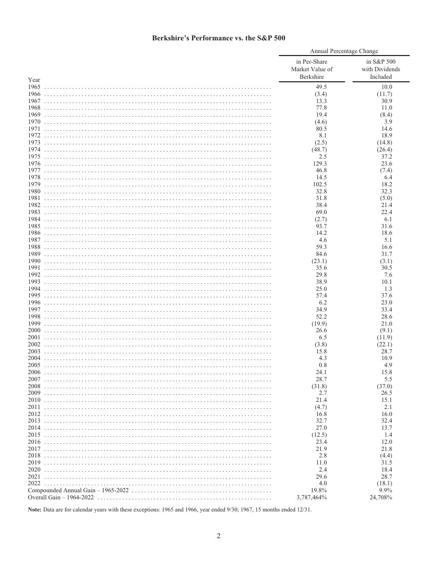 巴菲特致股东的公开信 - 2022.pdf
 MySQL 8.1 参考手册.pdf
 世界银行报告下载:激进政策缩紧浪潮不足遏制通胀 全球经济衰退迫在眉睫(Is a Global Recession Imminent?).pdf
 红杉资本报告:适应与忍耐(Adapting to Endure).pdf
 高保真音响系统设计制作-毕业论文.doc
 一种自适应互补滤波姿态估计算法.pdf