An efficient orientation filter for inertial and
inertial/magnetic sensor arrays
Sebastian O.H. Madgwick
April 30, 2010
Abstract
This report presents a novel orientation filter applicable to IMUs consisting of
tri-axis gyroscopes and accelerometers, and MARG sensor arrays that also include
tri-axis magnetometers. The MARG implementation incorporates magnetic distortion
and gyroscope bias drift compensation. The filter uses a quaternion representation,
allowing accelerometer and magnetometer data to be used in an analytically derived
and optimised gradient-descent algorithm to compute the direction of the gyroscope
measurement error as a quaternion derivative. The benefits of the filter include: (1)
computationally inexpensive; requiring 109 (IMU) or 277 (MARG) scalar arithmetic
operations each filter update, (2) effective at low sampling rates; e.g. 10 Hz, and (3)
contains 1 (IMU) or 2 (MARG) adjustable parameters defined by observable system
characteristics. Performance was evaluated empirically using a commercially available
orientation sensor and reference measurements of orientation obtained using an optical
measurement system. A simple calibration method is presented for the use of the
optical measurement equipment in this application. Performance was also benchmarked
against the propriety Kalman-based algorithm of orientation sensor. Results indicate
the filter achieves levels of accuracy exceeding that of the Kalman-based algorithm;
< 0.6◦ static RMS error, < 0.8◦ dynamic RMS error. The implications of the low
computational load and ability to operate at low sampling rates open new opportunities
for the use of IMU and MARG sensor arrays in real-time applications of limited power
or processing resources or applications that demand extremely high sampling rates.
1
�
Contents
1 Introduction
2 Quaternion representation
3 Filter derivation
3.1 Orientation from angular rate . . . . . . . . . . . . . . . . . . . . . . . . . .
3.2 Orientation from vector observations
. . . . . . . . . . . . . . . . . . . . . .
3.3 Filter fusion algorithm . . . . . . . . . . . . . . . . . . . . . . . . . . . . . .
3.4 Magnetic distortion compensation . . . . . . . . . . . . . . . . . . . . . . . .
3.5 Gyroscope bias drift compensation . . . . . . . . . . . . . . . . . . . . . . .
. . . . . . . . . . . . . . . . . . . . . . . . . . . . . . . . . . . .
3.6 Filter gains
4 Experimentation
4.1 Equipment . . . . . . . . . . . . . . . . . . . . . . . . . . . . . . . . . . . . .
4.2 Orientation from optical measurements . . . . . . . . . . . . . . . . . . . . .
4.3 Calibration of frame alignments . . . . . . . . . . . . . . . . . . . . . . . . .
4.4 Experimental proceedure . . . . . . . . . . . . . . . . . . . . . . . . . . . . .
5 Results
5.1 Typical results
. . . . . . . . . . . . . . . . . . . . . . . . . . . . . . . . . .
5.2 Static and dynamic performance
. . . . . . . . . . . . . . . . . . . . . . . .
5.3 Filter gain vs. performance . . . . . . . . . . . . . . . . . . . . . . . . . . . .
5.4 Sampling rate vs. performance . . . . . . . . . . . . . . . . . . . . . . . . . .
5.5 Gyroscope bias drift
. . . . . . . . . . . . . . . . . . . . . . . . . . . . . . .
6 Discussion
7 Conclusions
A IMU filter implementation optimised in C
B MARG filter implementation optimised in C
3
4
6
6
6
10
11
12
13
14
14
14
16
18
19
19
21
22
23
23
24
25
29
30
2
�
1
Introduction
The accurate measurement of orientation plays a critical role in a range of fields includ-
ing: aerospace [1, 2, 3], robotics [4, 5], navigation [6, 7] and human motion analysis [8, 9]
and machine interaction [10]. Whilst a variety of technologies enable the measurement of
orientation, inertial based sensory systems have the advantage of being completely self con-
tained such that the measurement entity is constrained neither in motion nor to any specific
environment or location. An IMU (Inertial Measurement Unit) consists of gyroscopes and
accelerometers enabling the tracking of rotational and translational movements. In order to
measure in three dimensions, tri-axis sensors consisting of 3 mutually orthogonal sensitive
axes are required. A MARG (Magnetic, Angular Rate, and Gravity) sensor is a hybrid IMU
which incorporates a tri-axis magnetometer. An IMU alone can only measure an attitude
relative to the direction of gravity which is sufficient for many applications [4, 2, 8, 1]. MARG
systems, also known as AHRS (Attitude and Heading Reference Systems) are able to provide
a complete measurement of orientation relative to the direction of gravity and the earth’s
magnetic field.
A gyroscope measures angular velocity which, if initial conditions are known, may be inte-
grated over time to compute the sensor’s orientation [11, 12]. Precision gyroscopes, ring laser
for example, are too expensive and bulky for most applications and so less accurate MEMS
(Micro Electrical Mechanical System) devices are used in a majority of applications [13]. The
integration of gyroscope measurement errors will lead to an accumulating error in the calcu-
lated orientation. Therefore, gyroscopes alone cannot provide an absolute measurement of
orientation. An accelerometer and magnetometer will measure the earth’s gravitational and
magnetic fields respectively and so provide an absolute reference of orientation. However,
they are likely to be subject to high levels of noise; for example, accelerations due to motion
will corrupt measured direction of gravity. The task of an orientation filter is to compute
a single estimate of orientation through the optimal fusion of gyroscope, accelerometer and
magnetometer measurements.
The Kalman filter [14] has become the accepted basis for the majority of orientation filter
algorithms [4, 15, 16, 17] and commercial inertial orientation sensors; xsens [18], micro-strain
[19], VectorNav [20], Intersense [21], PNI [22] and Crossbow [23] all produce systems founded
on its use. The widespread use of Kalman-based solutions are a testament to their accuracy
and effectiveness, however, they have a number of disadvantages. They can be complicated to
implement which is reflected by the numerous solutions seen in the subject literature [3, 4, 15,
16, 17, 24, 25, 26, 27, 28, 29, 30, 31, 32]. The linear regression iterations, fundamental to the
Kalman process, demand sampling rates far exceeding the subject bandwidth; for example, a
sampling rate between 512 Hz [18] and 30 kHz [19] may be used for a human motion caption
application. The state relationships describing rotational kinematics in three-dimensions
typically require large state vectors and an extended Kalman filter implementation [4, 17, 24]
to linearise the problem.
These challenges demand a large computational load for implementation of Kalman-
based solutions and provide a clear motivation for alternative approaches. Many previous
approaches to address these issues have implemented either fuzzy processing [2, 5] or fixed
filters [33] to favour accelerometer measurements of orientation at low angular velocities and
the integrated gyroscope measurements at high angular velocities. Such an approach is simple
3
�
but may only be effective under limited operating conditions. Bachman et al [34] proposed
an alternative approach where the filter achieves an optimal fusion of measurements data at
all angular velocities. However, the process requires a least squares regression, which also
brings in an associated computational load. Mahony et al [35] developed the complementary
filter which is shown to be an efficient and effective solution; however, performance is only
validated for an IMU.
This report introduces novel orientation filter that is applicable to both IMUs and MARG
sensor arrays addressing issues of computational load and parameter tuning associated with
Kalman-based approaches. The filter employs a quaternion representation of orientation (as
in: [34, 17, 24, 30, 32]) to describe the coupled nature of orientations in three-dimensions and
is not subject to the problematic singularities associated with an Euler angle representation1.
A complete derivation and empirical evaluation of the new filter is presented. Its performance
is benchmarked against an existing commercial filter and verified with optical measurement
system.
Innovative aspects of the proposed filter include: a single adjustable parameter
defined by observable systems characteristics; an analytically derived and optimised gradient-
descent algorithm enabling performance at low sampling rates; an on-line magnetic distortion
compensation algorithm; and gyroscope bias drift compensation.
2 Quaternion representation
A quaternion is a four-dimensional complex number that can be used to represent the ori-
entation of a ridged body or coordinate frame in three-dimensional space. An arbitrary
orientation of frame B relative to frame A can be achieved through a rotation of angle θ
around an axis A ˆr defined in frame A. This is represented graphically in figure 1 where the
mutually orthogonal unit vectors ˆxA, ˆyA and ˆzA, and ˆxB, ˆyB and ˆzB define the principle axis
of coordinate frames A and B respectively. The quaternion describing this orientation, A
B ˆq,
is defined by equation (1) where rx, ry and rz define the components of the unit vector A ˆr in
the x, y and z axes of frame A respectively. A notation system of leading super-scripts and
sub-scripts adopted from Craig [37] is used to denote the relative frames of orientations and
vectors. A leading sub-script denotes the frame being described and a leading super-script
denotes the frame this is with reference to. For example, A
B ˆq describes the orientation of
frame B relative to frame A and A ˆr is a vector described in frame A. Quaternion arithmetic
often requires that a quaternion describing an orientation is first normalised. It is therefore
conventional for all quaternions describing an orientation to be of unit length.
A
B ˆq =q1
q4 =cos θ
q2
q3
(1)
The quaternion conjugate, denoted by ∗, can be used to swap the relative frames described
B ˆq and describes the orientation of
A ˆq is the conjugate of A
by an orientation. For example, B
frame A relative to frame B. The conjugate of A
2 −rxsin θ
2 −rysin θ
B ˆq is defined by equation (2).
2
2 −rzsin θ
1Kuipers [36] offers a comprehensive introduction to this use of quaternions.
∗ = B
A
B ˆq
A ˆq =q1 −q2 −q3 −q4
(2)
4
�
Figure 1: The orientation of frame B is achieved by a rotation, from alignment with frame
A, of angle θ around the axis Ar.
The quaternion product, denoted by ⊗, can be used to define compound orientations.
C ˆq, the compounded orientation A
C ˆq
B ˆq and B
For example, for two orientations described by A
can be defined by equation (3).
A
C ˆq = B
C ˆq ⊗ A
B ˆq
For two quaternions, a and b, the quaternion product can be determined using the
Hamilton rule and defined as equation (4). A quaternion product is not commutative; that
is, a ⊗ b = b ⊗ a.
a ⊗ b =a1 a2 a3 a4 ⊗b1
=
b2
a1b1 − a2b2 − a3b3 − a4b4
a1b2 + a2b1 + a3b4 − a4b3
a1b3 − a2b4 + a3b1 + a4b2
a1b4 + a2b3 − a3b2 + a4b1
b3
T
b4
(4)
A three dimensional vector can be rotated by a quaternion using the relationship de-
scribed in equation (5) [36]. Av and Bv are the same vector described in frame A and frame
B respectively where each vector contains a 0 inserted as the first element to make them 4
element row vectors.
(3)
(5)
(6)
Bv = A
∗
B ˆq ⊗ Av ⊗ A
B ˆq
The orientation described by A
B ˆq can be represented as the rotation matrix A
BR defined
by equation (6) [36].
A
BR =
2
2q2
1 − 1 + 2q2
2(q2q3 − q1q4) 2q2
2(q2q4 + q1q3) 2(q3q4 − q1q2) 2q2
2(q2q3 + q1q4) 2(q2q4 − q1q3)
2(q3q4 + q1q2)
1 − 1 + 2q2
1 − 1 + 2q2
3
4
Euler angles ψ, θ and φ in the so called aerospace sequence [36] describe an orientation
of frame B achieved by the sequential rotations, from alignment with frame A, of ψ around
5
ˆyAˆyBAˆrˆxBˆxAθˆzAˆzB�
ˆzB, θ around ˆyB, and φ around ˆxB. This Euler angle representation of A
equations (7), (8) and (9).
B ˆq is defined by
ψ = Atan22q2q3 − 2q1q4, 2q2
1 + 2q2
θ = −sin−1 (2q2q4 + 2q1q3)
φ = Atan22q3q4 − 2q1q2, 2q2
1 + 2q2
2 − 1
4 − 1
(7)
(8)
(9)
3 Filter derivation
3.1 Orientation from angular rate
A tri-axis gyroscope will measure the angular rate about the x, y and z axes of the senor
frame, termed ωx, ωy and ωz respectively. If these parameters (in rads−1) are arranged into
the vector Sω defined by equation (10), the quaternion derivative describing the rate of
change of orientation of the earth frame relative to the sensor frame S
E ˙q can be calculated
[38] as equation (11).
Sω =0 ωx ωy ωz
E ˆq ⊗ Sω
S
E ˙q =
1
2
S
(10)
(11)
The orientation of the earth frame relative to the sensor frame at time t, E
S qω,t, can
be computed by numerically integrating the quaternion derivative S
E ˙qω,t as described by
equations (12) and (13) provided that initial conditions are known. In these equations, Sωt
is the angular rate measured at time t, ∆t is the sampling period and S
E ˆqest,t-1 is the previous
estimate of orientation. The sub-script ω indicates that the quaternion is calculated from
angular rates.
S
E ˙qω,t =
1
2
S
E ˆqest,t-1 ⊗ Sωt
Eqω,t = S
S
E ˆqest,t-1 + S
E ˙qω,t∆t
(12)
(13)
3.2 Orientation from vector observations
A tri-axis accelerometer will measure the magnitude and direction of the field of gravity in the
sensor frame compounded with linear accelerations due to motion of the sensor. Similarly, a
tri-axis magnetometer will measure the magnitude and direction of the earth’s magnetic field
in the sensor frame compounded with local magnetic flux and distortions. In the context
of an orientation filter, it will initially be assumed that an accelerometer will measure only
gravity, a magnetometer will measure only the earth’s magnetic field.
6
�
If the direction of an earth’s field is known in the earth frame, a measurement of the
field’s direction within the sensor frame will allow an orientation of the sensor frame relative
to the earth frame to be calculated. However, for any given measurement there will not be
a unique sensor orientation solution, instead there will infinite solutions represented by all
those orientations achieved by the rotation the true orientation around an axis parallel with
the field. In some applications it may be acceptable to use an Euler angle representation
allowing an incomplete solution to be found as two known Euler angles and one unknown [5];
the unknown angle being the rotation around an axis parallel with the direction of the field.
A quaternion representation requires a complete solution to be found. This may be achieved
through the formulation of an optimisation problem where an orientation of the sensor, S
E ˆq,
is that which aligns a predefined reference direction of the field in the earth frame, E ˆd,
with the measured direction of the field in the sensor frame, S ˆs, using the rotation operation
described by equation (5). Therefore S
E ˆq may be found as the solution to (14) where equation
(15) defines the objective function. The components of each vector are defined in equations
(16) to (18).
f (S
E ˆq, E ˆd, S ˆs) = S
f (S
E ˆq, E ˆd, S ˆs)
min
E ˆq∈4
S
∗
E ˆq
S
q2
⊗ E ˆd ⊗ S
E ˆq − S ˆs
q4
E ˆq =q1
q3
E ˆd =0 dx dy dz
S ˆs =0 sx sy sz
(14)
(15)
(16)
(17)
(18)
Many optimisation algorithms exist but the gradient descent algorithm is one of the
simplest to both implement and compute. Equations (19) describes the gradient descent
algorithm for n iterations resulting in an orientation estimation of S
E ˆqn+1 based on an ‘initial
guess’ orientation S
E ˆq0 and a step-size µ. Equation (20) computes the gradient of the solution
surface defined by the objective function and its Jacobian; simplified to the 3 row vectors
defined by equations (21) and (22) respectively.
S
Eqk+1 = S
E ˆqk, E ˆd, S ˆs)
E ˆqk − µ ∇f (S
∇f (S
E ˆqk, E ˆd, S ˆs)
E ˆqk, E ˆd, S ˆs) = J T (S
E ˆqk, E ˆd)f (S
∇f (S
, k = 0, 1, 2...n
E ˆqk, E ˆd, S ˆs)
f (S
E ˆqk, E ˆd, S ˆs) =
3 − q2
2 − q2
2 − q2
2dx( 1
4) + 2dy(q1q4 + q2q3)+
2dx(q2q3 − q1q4) + 2dy( 1
4)+
2dx(q1q3 + q2q4) + 2dy(q3q4 − q1q2)+
2dz(q2q4 − q1q3) − sx
2dz(q1q2 + q3q4) − sy
2dz( 1
3) − sz
2 − q2
2 − q2
2 − q2
7
(19)
(20)
(21)
�
J (S
E ˆqk, E ˆd) =
2dyq3 + 2dzq4
2dyq4 − 2dzq3
−2dxq4 + 2dzq2 2dxq3 − 4dyq2 + 2dzq1
2dxq4 − 2dyq1 − 4dzq2
2dxq3 − 2dyq2
−4dxq3 + 2dyq2 − 2dzq1 −4dxq4 + 2dyq1 + 2dzq2
−2dxq1 − 4dyq4 + 2dzq3
2dxq1 + 2dyq4 − 4dzq3
2dxq2 + 2dyq3
2dxq2 + 2dzq4
Equations (19) to (22) describe the general form of the algorithm applicable to a field
predefined in any direction. However, if the direction of the field can be assumed to only
have components within 1 or 2 of the principle axis of the global coordinate frame then
the equations simplify. An appropriate convention would be to assume that the direction of
gravity defines the vertical, z axis as shown in equation (23). Substituting E ˆg and normalised
accelerometer measurement S ˆa for E ˆd and S ˆs respectively, in equations (21) and (22) yields
equations (25) and (26).
E ˆg =0 0 0 1
S ˆa =0 ax ay az
E ˆq, S ˆa) =
E ˆq) =
2(q2q4 − q1q3) − ax
2(q1q2 + q3q4) − ay
2( 1
2 − q2
3) − az
2q4 −2q1 2q2
2q3
2q1
2q4
−4q2 −4q3
−2q3
2q2
0
2 − q2
0
fg(S
Jg(S
(22)
(23)
(24)
(25)
(26)
The earth’s magnetic field can be considered to have components in one horizontal axis
and the vertical axis; the vertical component due to the inclination of the field which is
between 65◦ and 70◦ to the horizontal in the UK [39]. This can be represented by equa-
tion (27). Substituting Eˆb and normalised magnetometer measurement S ˆm for E ˆd and S ˆs
respectively, in equations (21) and (22) yields equations (29) and (30).
Eˆb =0 bx 0 bz
S ˆm =0 mx my mz
fb(S
E ˆq, Eˆb, S ˆm) =
3 − q2
2bx(0.5 − q2
4) + 2bz(q2q4 − q1q3) − mx
2bx(q2q3 − q1q4) + 2bz(q1q2 + q3q4) − my
2bx(q1q3 + q2q4) + 2bz(0.5 − q2
3) − mz
2 − q2
(27)
(28)
(29)
8
�


 2025年软考高级信息系统项目管理师金色考点
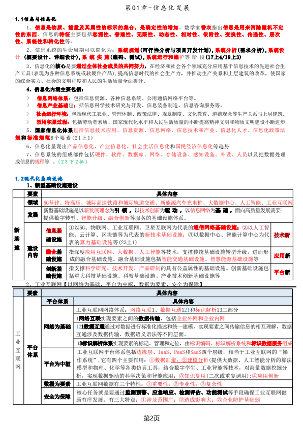 软考高项三色笔记
 镇安县双鑫矿业月河年处理15万吨尾渣综合加工利用项目水土保持报告表
  红杉资本:生成式AI最新市场格局.pdf
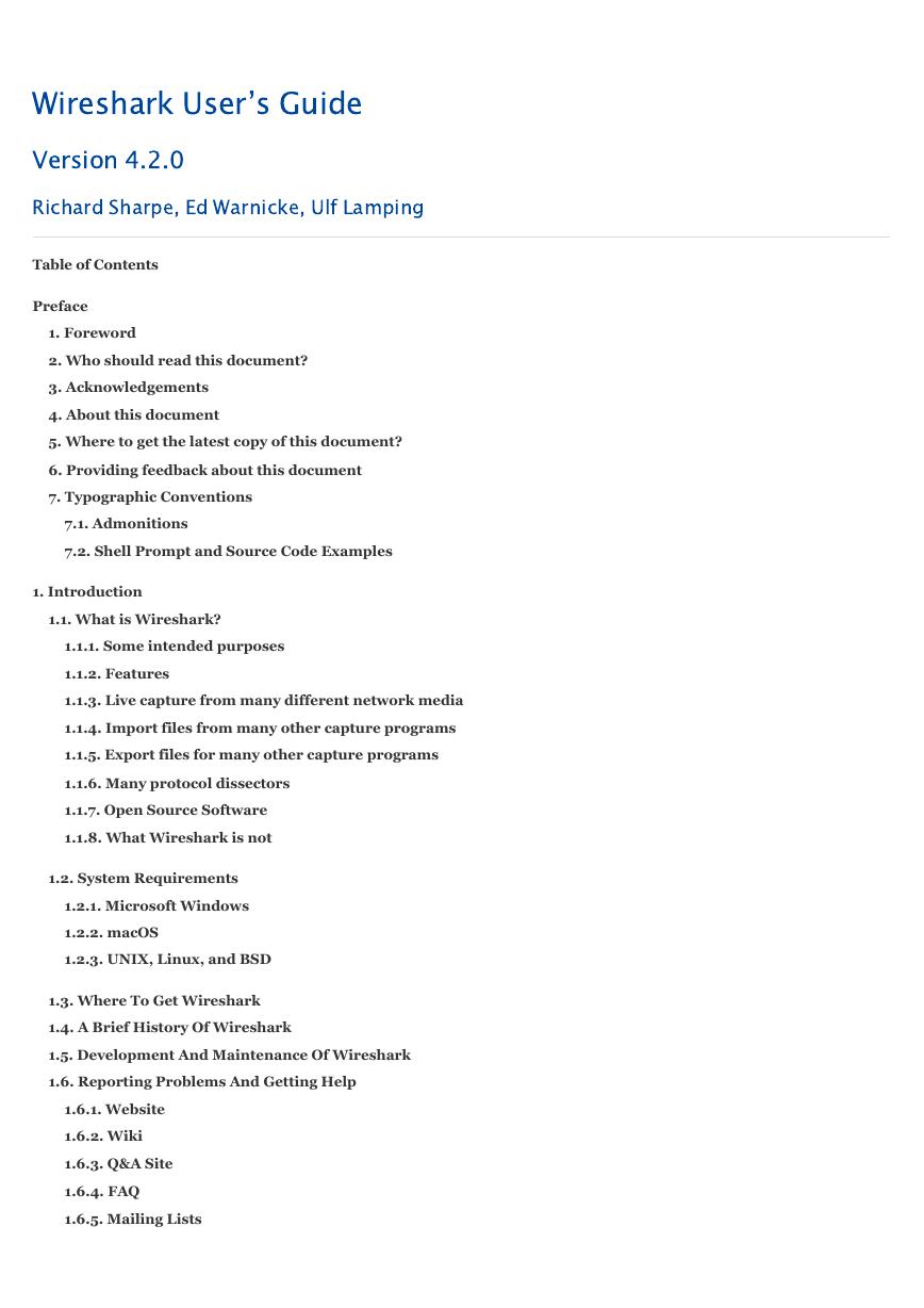 wireshark 使用教程.pdf
 【2021年-贝佐斯致股东的信】.pdf
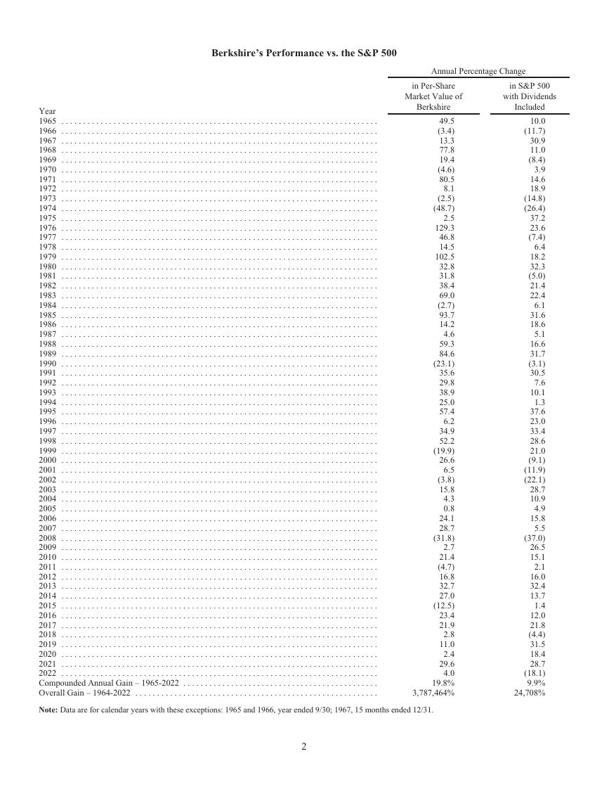 巴菲特致股东的公开信 - 2022.pdf
 MySQL 8.1 参考手册.pdf
 世界银行报告下载:激进政策缩紧浪潮不足遏制通胀 全球经济衰退迫在眉睫(Is a Global Recession Imminent?).pdf
 红杉资本报告:适应与忍耐(Adapting to Endure).pdf
 高保真音响系统设计制作-毕业论文.doc
 一种自适应互补滤波姿态估计算法.pdf